Plots#

Visualization Module#

This module provides visualization tools for analyzing and understanding the dynamics of adaptive environments and agent interactions for influencer games. It includes plotting utilities for various domains (1D, 2D, and simplex) and supports visualizing agent positions, gradients, influence distributions, and bifurcation dynamics.

The module is designed to work with the AdaptiveEnv class and provides a framework for creating visual representations of agent behaviors in influencer game environments.

Dependencies:#

InflGame.utils
InflGame.kernels
InflGame.domains

Usage:#

The Shell class can be used to visualize the results of simulations performed using the AdaptiveEnv class. It supports various visualization types, including position plots, gradient plots, probability plots, and bifurcation plots.

Examples#

from InflGame.adaptive.visualization import Shell
import torch
import numpy as np

# Initialize the Shell
shell = Shell(
    num_agents=3,
    agents_pos=np.array([0.2, 0.5, 0.8]),
    parameters=torch.tensor([1.0, 1.0, 1.0]),
    resource_distribution=torch.tensor([10.0, 20.0, 30.0]),
    bin_points=np.array([0.1, 0.4, 0.7]),
    infl_configs={'infl_type': 'gaussian'},
    learning_rate_type='cosine_annealing',
    learning_rate=[0.0001, 0.01, 15],
    time_steps=100,
    domain_type='1d',
    domain_bounds=[0, 1]
)

# Set up the adaptive environment
shell.setup_adaptive_env()

# Plot agent positions
fig = shell.pos_plot()
fig.show()

Classes

class InflGame.adaptive.visualization.Shell(num_agents, agents_pos, parameters, resource_distribution, bin_points, infl_configs={'infl_type': 'gaussian'}, learning_rate_type='cosine_annealing', learning_rate=[0.0001, 0.01, 15], time_steps=100, fp=0, infl_cshift=False, cshift=None, infl_fshift=False, Q=None, domain_type=None, rect_X=None, rect_Y=None, rect_positions=None, resource_grid=None, domain_bounds=[0, 1], resource_type='na', domain_refinement=10, tolerance=1e-05, tolerated_agents=None, ignore_zero_infl=False, device=None)#

The Shell class provides a framework for simulating and visualizing adaptive dynamics in various domains (1D, 2D, and simplex). It supports gradient ascent, influence distribution calculations, and plotting utilities for analyzing agent behaviors in resource distribution environments.

Methods

`agent_density_3d`([pos_matrix, bins, ...])	Create a 3D histogram showing agent counts at final positions.
`analyze_near_critical_point`(x_star[, ...])	Perform high-resolution analysis near the theoretical critical point x*.
`analyze_zero_crossings`(refined_parameters, ...)	Perform detailed analysis of zero crossings in the refined parameter space.
`bifurcation_plot_AD_MARL`(parameters_AD, ...)	Create side-by-side bifurcation plots comparing Adaptive Dynamics (AD) and Multi-Agent Reinforcement Learning (MARL) approaches.
`bifurcation_tree`(main_matrix, left_matrices, ...)	Create a vertical tree plot with a main rectangle and left/right branches based on bifurcation changes.
`calc_direction_and_strength`([...])	Calculate the direction and strength of gradients for agents via interacting with `InflGame.adaptive.grad_func_env` .
`calc_infl_dist`(pos, parameter_instance)	Calculate the influence distribution for agents via thier influence kernels by interacting with the class `InflGame.adaptive.grad_func_env` .
`dist_plot`(agent_id[, parameter_instance, ...])	Plot the agents' influence distributions distributions via the function `calc_infl_dist` .
`dist_pos_gif`(max_frames[, x_min, y_min, ...])	Plot the agents' influence distributions and their positions into a gif.
`dist_pos_plot`(parameter_instance[, ...])	Plots the agents' influence distributions with their their positions.
`equilibrium_bifurcation_plot`([matrix, ...])	Plots the equilibrium bifurcation for agents over a range of reach parameters.
`find_and_analyze_zero_crossings`(test_eval, ...)	Complete workflow to find, refine, and analyze eigenvalue zero crossings.
`find_zero_crossings`(test_eval, parameters_list)	Identify parameter values where eigenvalue real parts are close to zero.
`first_order_bifurcation_plot`(processed_data)	Generate and plot first-order bifurcation diagram with stability analysis.
`first_order_bifurcation_plot_old`(...[, ...])	Plots the first-order bifurcation for agents over a range of alpha values (resource parameters) via func:`jacobian_stability_fast`.
`generate_combined_figure`(alpha, ...[, ...])	Generate the standardized combined bifurcation and equilibrium analysis figure.
`grad_plot`([title_ads, save, name_ads, font, ...])	Plots the gradients of agents as the lines versus time.
`jacobian_stability_fast`(...[, ...])	Calculate the stability of the symmetric Nash equilibrium via analytical computation of maximum eigenvalues.
`node_to_images`(main, left_matrices, ...[, ...])	process all matrices and create images for each node
`plot_equilibrium_heatmap`(newton_search_data)	Generate and plot a heatmap of equilibrium positions in a 1D influence game.
`pos_plot`([title_ads, fig_size, save, ...])	Plots the positions of agents over gradient ascent steps.
`position_at_equalibirum_histogram`([...])	Plot the histogram of agents' positions at equilibrium for a given reach parameter via the function `InflGame.adaptive.grad_func_env.gradient_ascent` .
`prob_plot`([position, parameters, title_ads, ...])	Plot the probability distribution of agents' influence over a bin/resource point via their relative influence over that point
`resource_distribution_plot`([alpha, ...])	Plots the resource distribution with optional alpha line annotation for bimodal distributions.
`reward_groups_stacked`([idx, rwd_type, ...])	Plot stacked reward groups across agents for a selected bifurcation slice.
`setup_adaptive_env`()	Set up the adaptive environment for the simulation.
`setup_bifurcation_env`()	Set up the bifurcation environment for parameter sweep analysis.
`simple_diagonal_test_point`([point])	Test a single point to verify gradient ascent functionality.
`three_agent_pos_3A1d`([x_star, title_ads, ...])	Create combined visualization showing three-agent dynamics in 3D space alongside position trajectories.
`three_agent_pos_3d`([x_star, title_ads, ...])	Visualize dynamics for three players: demonstrates the players positions changing in time in 3-d space.
`threed_fixed_diagonal_view`([resolution, ...])	Creates a 3D plot with fixed view looking down the x=y=z diagonal line, showing gradient ascent trajectories from multiple starting points with optional parallel processing.
`threed_fixed_diagonal_view_gif`(max_frames[, ...])	Create a 3D diagonal view GIF showing gradient ascent traces over varying reach parameters.
`threed_gradient_ascent_paths_interactive`([...])	Creates an interactive 3D plot of gradient ascent paths from multiple starting points, with paths color-coded based on the initial position's quadrant.
`vect_plot`([agent_id, parameter_instance, ...])	Plot the vector field of gradients for a specific agents calculated by the function `calc_direction_and_strength` .

reward_bifurcation_matrix_setup

agent_density_3d(pos_matrix=None, bins=25, distance_threshold=0.05, cmap='viridis', font={'cbar_label_pad': 15, 'cbar_size': 16, 'default_size': 15, 'font_family': 'sans-serif', 'label_pad': 10, 'legend_size': 12, 'title_pad': 10, 'title_size': 18}, figsize=(20, 16), xlabel=None, ylabel=None, zlabel='Number of Agents', axis_return=False, edgecolor='black', linewidth=0.2, alpha=0.9, title_ads=[], save=False, name_ads=[], save_types=['.png', '.svg'], paper_figure={'figure_id': 'agent_density_3d', 'paper': False, 'section': 'A'}, id=0, cap_z_axis=True, integer_ticks=True)#

Create a 3D histogram showing agent counts at final positions.

Automatically selects the appropriate implementation based on domain type: - For ‘2d’ domains: Uses rectangular histogram binning - For ‘simplex’ domains: Converts barycentric to Cartesian and uses triangular binning with clustering

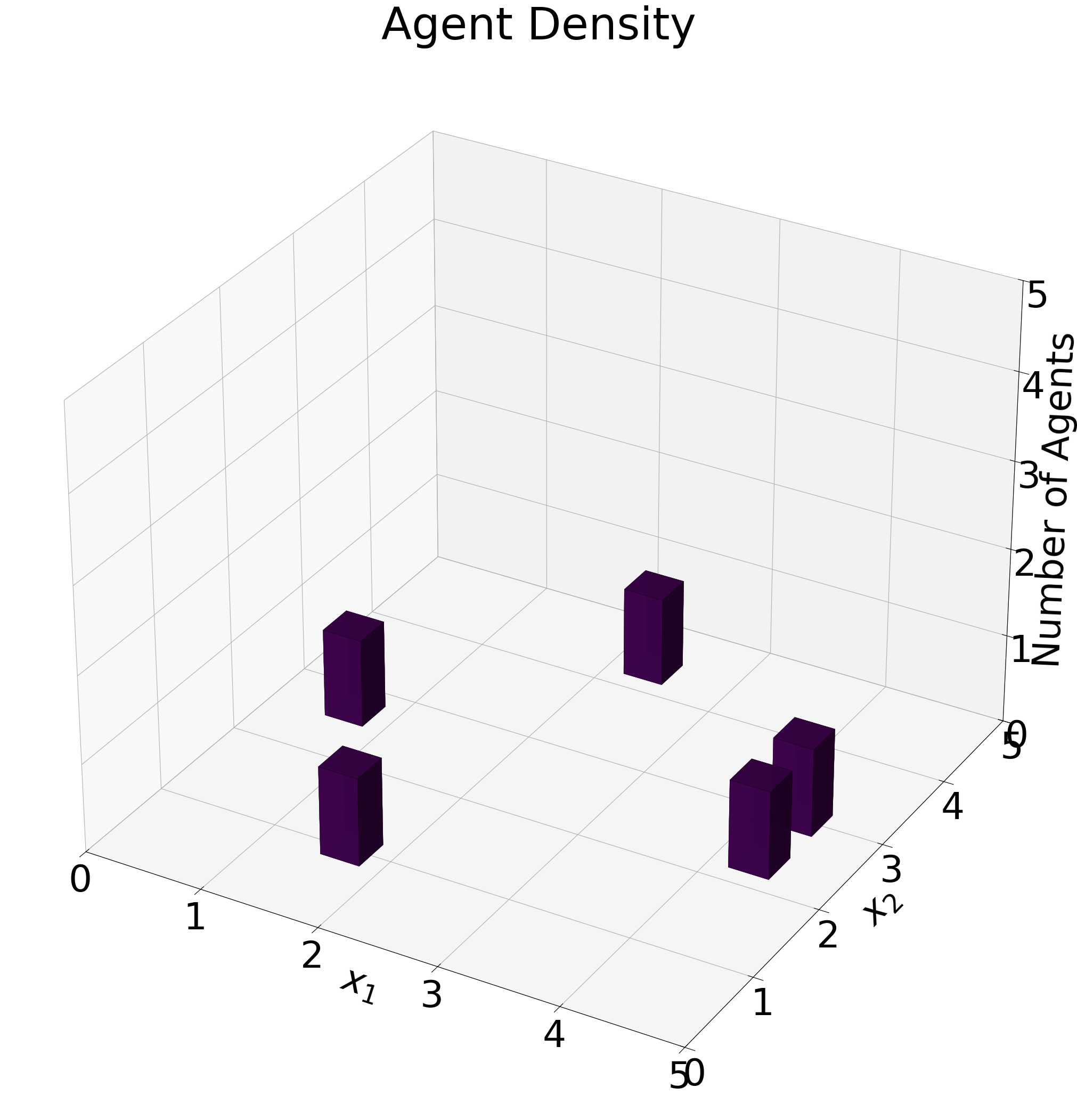
../../_images/agent_density_3d.png — Example agent-density histogram on the simplex.#

Parameters:

pos_matrixUnion[torch.Tensor, np.ndarray, None]: Position matrix. If None, uses self.field.pos_matrix.
binsint: Number of bins in each dimension.
distance_thresholdfloat: Distance threshold for clustering nearby agents (simplex only).
cmapstr: Colormap name.
fontdict: Font configuration dictionary.
figsizetuple: Figure size as (width, height).
xlabelstr: Label for x-axis.
ylabelstr: Label for y-axis.
zlabelstr: Label for z-axis.
axis_returnbool: If True, return axes object; if False, return figure object.
edgecolorOptional[str]: Color of outlines around bars.
linewidthfloat: Width of bar edge lines.
alphafloat: Bar transparency.
title_adsList[str]: Additional titles for the plot.
savebool: Whether to save the plot.
name_adsList[str]: Additional names for saved files.
save_typesList[str]: File types to save the plot.
paper_figuredict: Dictionary for paper figure naming.
idint: Identifier for file naming.
cap_z_axisbool: If True, cap the z-axis maximum at num_agents.
integer_ticksbool: If True, only show integer ticks on the z-axis.

Returns:

matplotlib.figure.Figure: The generated plot figure.

analyze_near_critical_point(x_star, padding=0.01, num_points=50)#

Perform high-resolution analysis near the theoretical critical point x*.

Parameters:

x_startorch.Tensor: Theoretical critical point.
paddingfloat: Range to examine on either side of x*.
num_pointsint: Number of parameter points to examine.

Returns:

dict: Analysis results focused on the critical point.

analyze_zero_crossings(refined_parameters, refined_eval, x_star=None)#

Perform detailed analysis of zero crossings in the refined parameter space.

Parameters:

refined_parameterstorch.Tensor: Tensor of refined parameter values.
refined_evaltorch.Tensor: Tensor of eigenvalues at refined parameters.
x_starOptional[torch.Tensor]: Theoretical critical point (if available).

Returns:

dict: Dictionary of analysis results and figure handles.

bifurcation_plot_AD_MARL(parameters_AD, parameters_MARL, matrix=None, fontmain={'axis_size': 15, 'cbar_size': 16, 'default_size': 15, 'font_family': 'sans-serif', 'legend_size': 12, 'title_size': 18}, save=False, name_ads=[], save_types=['.png', '.svg'], paper_figure={'figure_id': 'pos_plot', 'paper': False, 'section': 'A'}, envolve=False, complete=False, bifurcation_key_tolerance=3, show_legend=True, svg_options=None)#

Create side-by-side bifurcation plots comparing Adaptive Dynamics (AD) and Multi-Agent Reinforcement Learning (MARL) approaches.

This method generates comparative visualization showing how equilibrium positions change with parameter variation for both gradient-based adaptive dynamics and reinforcement learning methods.

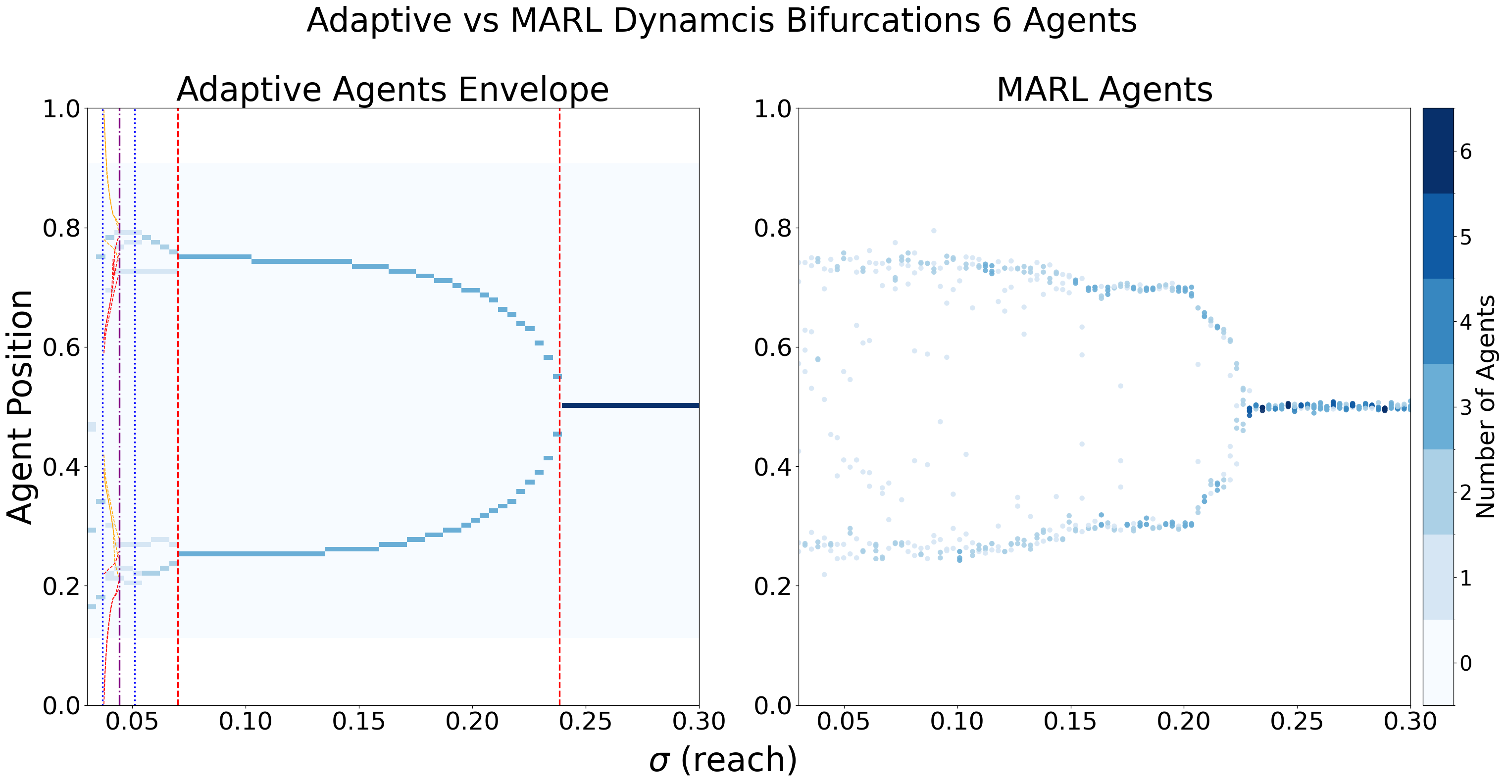
../../_images/bifurcation_ad_marl.png — Side-by-side AD vs MARL bifurcation comparison for five agents.#

Parameters:

parameters_ADdict: Configuration dictionary for adaptive dynamics bifurcation with keys: - ‘reach_start’: Starting reach parameter value - ‘reach_end’: Ending reach parameter value - ‘reach_num_points’: Number of parameter points - ‘time_steps’: Gradient ascent iterations - ‘tolerance’: Convergence tolerance - ‘tolerated_agents’: Number of agents for convergence check - ‘plot_type’: Type of bifurcation plot - ‘refinements’: Plot refinement level - ‘title_ads’: Additional title strings - ‘cmaps’: Color map configuration - ‘cbar_config’: Colorbar configuration - ‘parallel_configs’: Parallel processing settings - ‘font’: Font configuration
parameters_MARLdict: Configuration dictionary for MARL bifurcation with keys: - ‘step_size’: Step size for RL environment - ‘resource’: Resource distribution type - ‘reach_start’: Starting reach parameter - ‘reach_end’: Ending reach parameter - ‘reach_parameters’: Array of reach parameter values - ‘refinements’: Plot refinement level - ‘plot_type’: Type of bifurcation plot - ‘infl_type’: Influence kernel type - ‘title_ads’: Additional title strings - ‘font’: Font configuration - ‘cbar_config’: Colorbar configuration
fontmaindict: Main font configuration for combined plot.
savebool: Whether to save the plot.
name_adsList[str]: Additional filename components for saving.
save_typesList[str]: File formats for saving (e.g., [‘.png’, ‘.svg’]).
paper_figuredict: Paper figure configuration with ‘paper’, ‘section’, ‘figure_id’ keys.

Returns:

matplotlib.figure.Figure: Combined matplotlib figure with AD and MARL bifurcation plots.

bifurcation_tree(main_matrix, left_matrices, right_matrices, reach_start, reach_end, reach_num_points, label_to_color=None, figsize=(20, 24), rect_width=0.8, horizontal_spacing=2.5, box_height=10, box_width=0.1, key_tolerance=2, image_zoom=0.15, box_space=None, image_offset=(0, 0), branch_spacing=1.5, label_offset=0.1, show_labels=False, hide_text=False, max_reward=None, display_type='tree', title_ads=[], save=False, name_ads=[], font={'cbar_size': 16, 'default_size': 30, 'font_family': 'sans-serif', 'label_size': 10, 'legend_size': 12, 'table_size': 15, 'title_size': 60}, font_sub={'cbar_size': 16, 'default_size': 24, 'font_family': 'sans-serif', 'label_size': 24, 'legend_size': 12, 'table_size': 15, 'title_size': 32}, save_types=['.png', '.svg'], paper_figure={'figure_id': 'reward_groups_stacked', 'paper': False, 'section': '3_2_6'}, show_column_labels=True)#

Create a vertical tree plot with a main rectangle and left/right branches based on bifurcation changes.

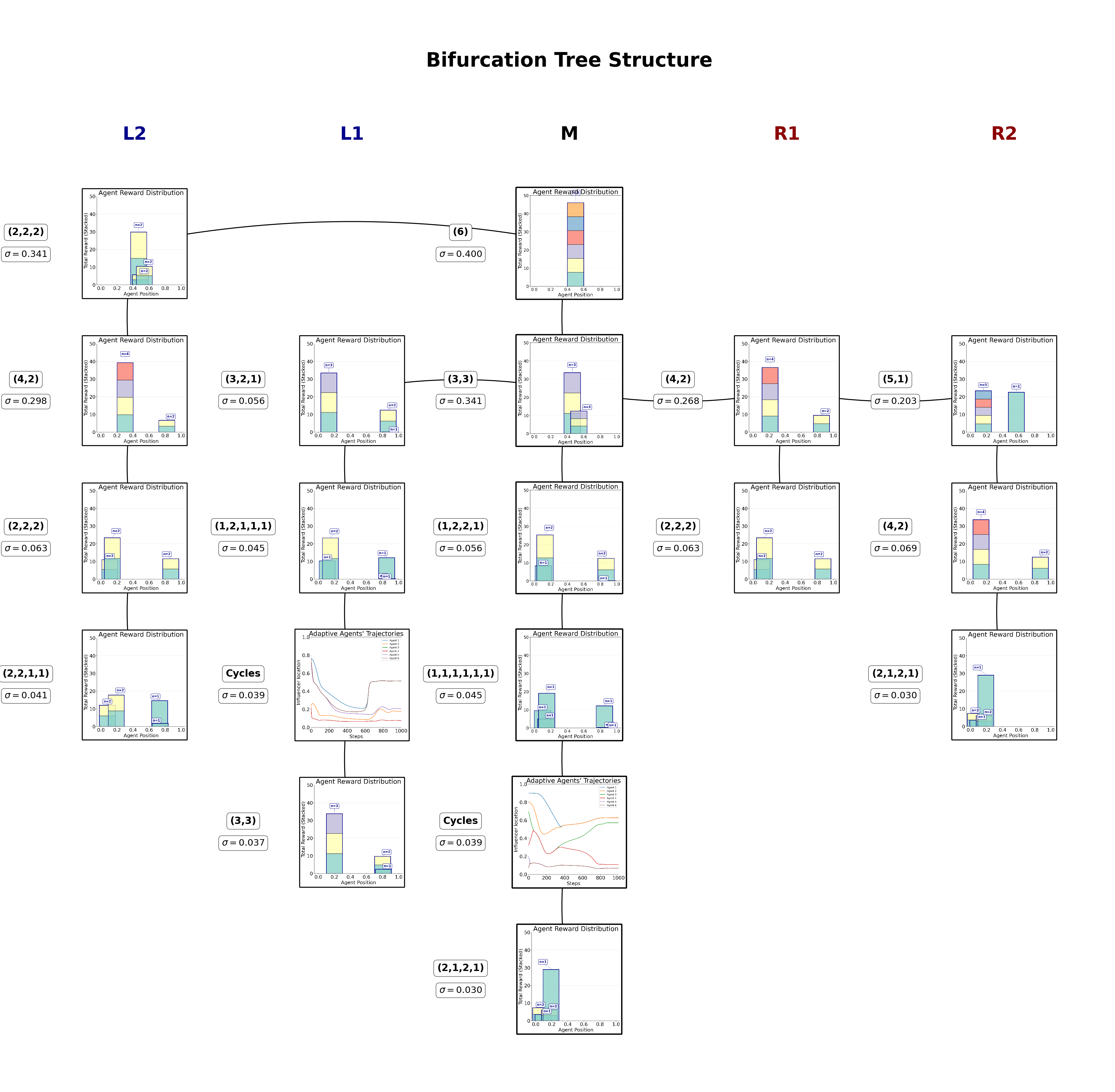
../../_images/bifurcation_tree.png — Example reward-annotated bifurcation tree for a six-player game.#

Parameters:

main_matrixdict: Main bifurcation matrix containing ‘max’, ‘min’, etc.
left_matriceslist of dict: List of matrices for left branches
right_matriceslist of dict: List of matrices for right branches
reach_parameterslist of torch.Tensor: Reach parameters for each matrix
num_agentsint: Number of agents in the system
reach_startfloat: Starting sigma value
reach_endfloat: Ending sigma value
label_to_colordict, optional: Mapping of classification labels to colors
figsizetuple: Figure size (width, height)
rect_widthfloat: Width of each rectangle
horizontal_spacingfloat: Spacing between rectangles
box_heightfloat: Total height of each rectangle
font_sizeint: Font size for labels
show_labelsbool: Whether to show classification labels on rectangles
display_typestr: ‘rect’ for rectangle display (colored rectangles with legends) ‘tree’ for tree display (text labels at branch points)

Returns:

fig, axmatplotlib figure and axes

calc_direction_and_strength(parameter_instance=0, agent_id=0, ids=[0, 1], pos=None, alt_form=False)#

Calculate the direction and strength of gradients for agents via interacting with InflGame.adaptive.grad_func_env .

Parameters:

parameter_instanceUnion[List[float], np.ndarray, torch.Tensor]: Parameters for the influence function.
agent_idint: ID of the agent.
idsList[int]: IDs of agents of interest.
posOptional[torch.Tensor]: Positions of agents.

Returns:

torch.Tensor: The calculated gradients.

calc_infl_dist(pos, parameter_instance)#

Calculate the influence distribution for agents via thier influence kernels by interacting with the class InflGame.adaptive.grad_func_env .

Parameters:

postorch.Tensor: Positions of agents.
parameter_instanceUnion[List[float], np.ndarray, torch.Tensor]: Parameters for the influence function.

Returns:

torch.Tensor: The influence distribution.

dist_plot(agent_id, parameter_instance=0, cmap='viridis', typelabels=['A', 'B', 'C'], save=False, name_ads=[], save_types=['.png', '.svg'], paper_figure={'figure_id': 'dist_plot', 'paper': False, 'section': 'A'}, font={'cbar_size': 16, 'default_size': 15, 'font_family': 'sans-serif', 'legend_size': 12, 'title_size': 18}, **kwargs)#

Plot the agents’ influence distributions distributions via the function calc_infl_dist .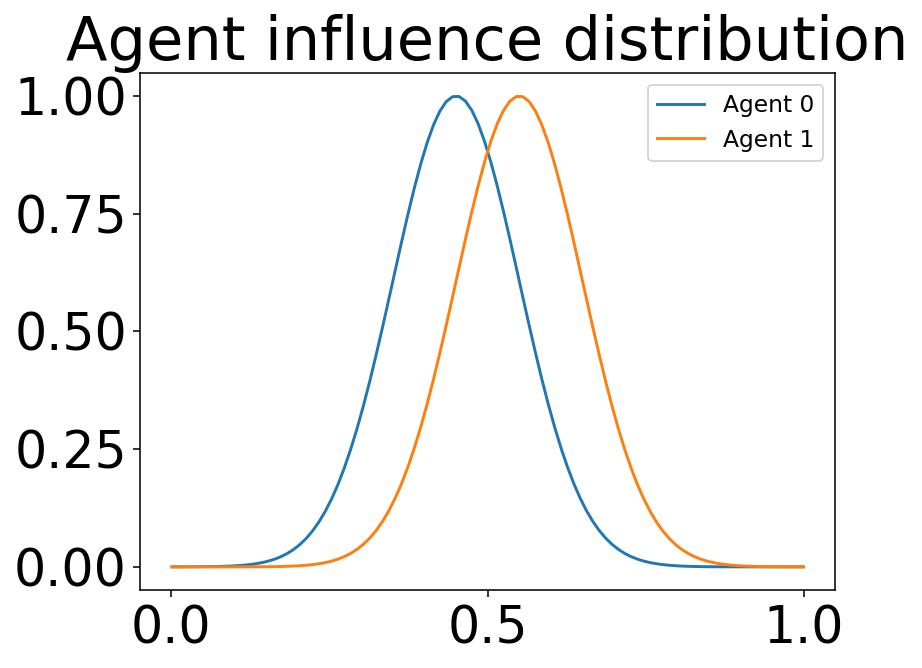

../../_images/dist_plot.png — Example 1D influence kernels for each agent.#

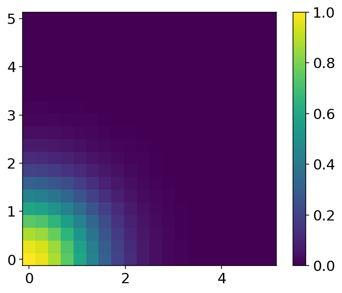
../../_images/dist_plot_2d.png — Example 2D influence distribution for a single agent.#

Parameters:

agent_idint: ID of the agent.
parameter_instanceUnion[List[float], np.ndarray, torch.Tensor]: Parameters for the influence function.
cmapstr: Colormap for the plot.
typelabelsList[str]: Labels for agent types.
kwargs: Additional arguments for plotting.

Returns:

matplotlib.figure.Figure: The generated plot figure.

dist_pos_gif(max_frames, x_min=None, y_min=None, output_filename='timelapse_test.gif', optimize_memory=True, dpi=100, fps=10, quality=8, verbose=False)#

Plot the agents’ influence distributions and their positions into a gif. Works for all domain types ‘1d’, ‘2d’, ‘simplex’. This is done by putting together frames of dist_pos_plot .

Optimized Performance Features: - Direct memory writing without intermediate files - Matplotlib figure recycling for memory efficiency - Optimized frame sampling - Configurable quality vs speed trade-offs

Simplex example

Simplex influence distribution and positions timelapse — This is a 3 player influence distribution and position plot gif for a simplex domain.#

Parameters:

max_framesint: Maximum number of frames for the gif.
output_filenamestr: Name of the output GIF file.
optimize_memorybool: Whether to use memory optimization techniques.
dpiint: DPI for the frames (lower = faster, higher = better quality).
fpsint: Frames per second for the GIF.
qualityint: GIF compression quality (1-10, lower = smaller file).
verbosebool: Whether to print progress information.

Returns:

matplotlib.figure.Figure: The generated gif figure.

dist_pos_plot(parameter_instance, typelabels=['A', 'B', 'C'], cmap1='twilight', cmap2='viridis', title_ads=[], save=False, name_ads=[], x_min=None, y_min=None, save_types=['.png', '.svg'], paper_figure={'figure_id': 'dist_pos_plot', 'paper': False, 'section': 'A'}, font={'cbar_size': 16, 'default_size': 15, 'font_family': 'sans-serif', 'legend_size': 12, 'title_size': 18})#

Plots the agents’ influence distributions with their their positions. The influence distributions are calculated from calc_infl_dist and the position vectors are calculated via InflGame.adaptive.grad_func_env.gradient_ascent . This function works with all 3 domain types ‘1d’,’2d’, and ‘simplex’.

** In one dimension**

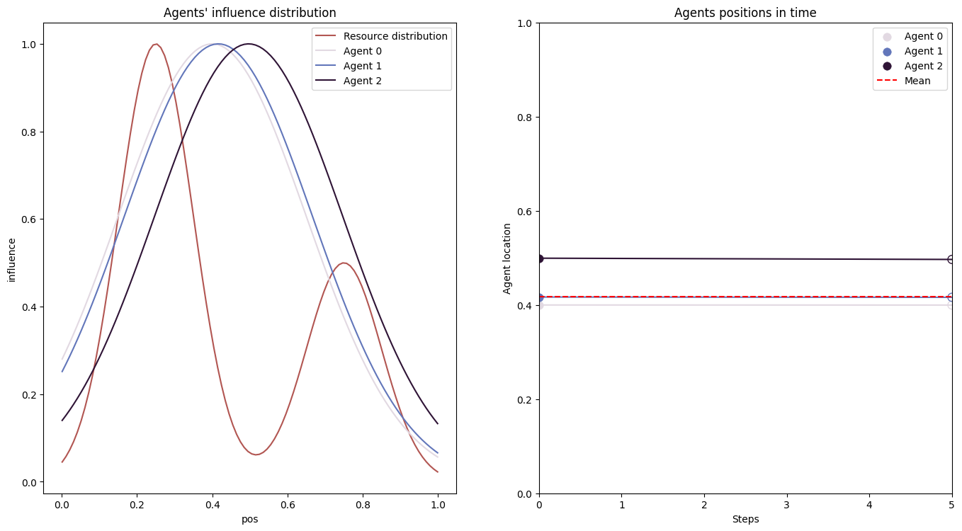
1D influence distribution and agent positions — This is a 3 player influence distribution and position plot for a 1d domain.#

For a simplex

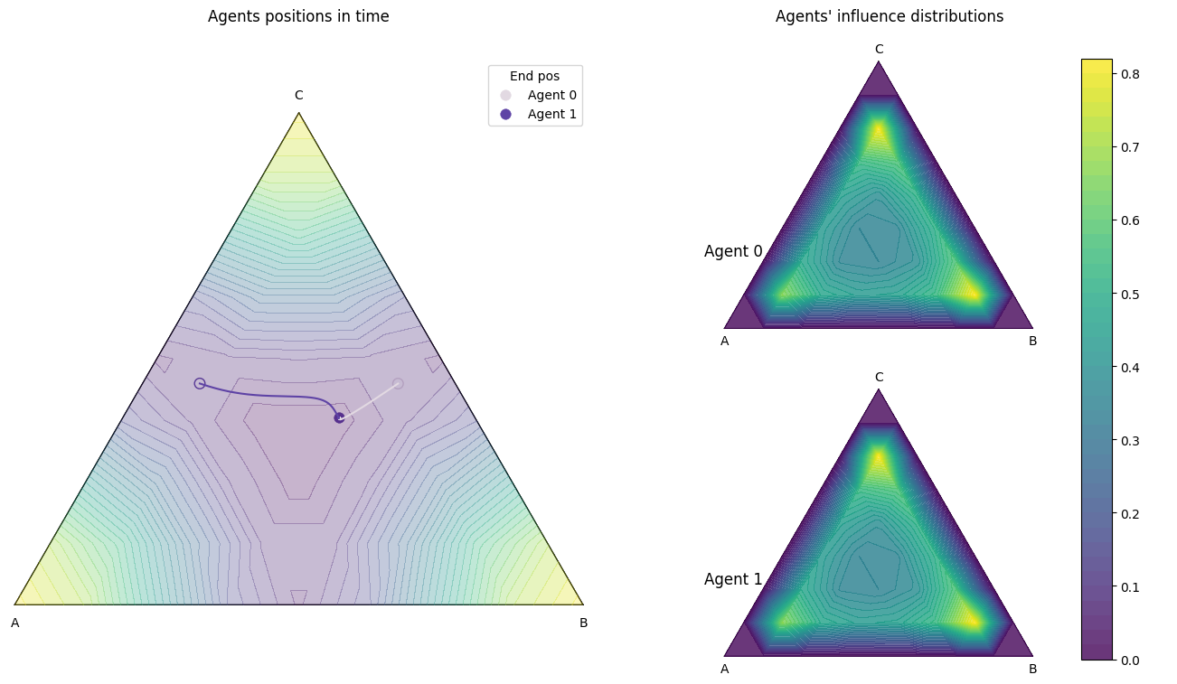
Simplex influence distribution and agent positions — This is a 2 player influence distribution and position plot for a simplex domain.#

Parameters:

parameter_instanceUnion[List[float], np.ndarray, torch.Tensor]: Parameters for the influence function.
typelabelsList[str]: Labels for agent types.
cmap1str: Colormap for the plot.
cmap2str: Colormap for the plot.
title_adsList[str]: Additional titles for the plot.
savebool: Whether to save the plot.
name_adsList[str]: Additional names for saved files.
save_typesList[str]: File types to save the plot.

Returns:

matplotlib.figure.Figure: The generated plot figure.

equilibrium_bifurcation_plot(matrix=None, reach_start=0.03, reach_end=0.3, reach_num_points=30, time_steps=100, initial_pos=None, current_alpha=0.5, tolerance=None, tolerated_agents=None, refinements=2, plot_type='heat', title_ads=[], name_ads=[], save=False, save_types=['.png', '.svg'], return_matrix=False, parallel_configs=None, cmaps={'crit': 'Greys', 'heat': 'Blues', 'trajectory': '#851321'}, font={'cbar_size': 16, 'default_size': 15, 'font_family': 'sans-serif', 'legend_size': 12, 'title_size': 18}, cbar_config={'center_labels': True, 'label_alignment': 'center', 'shrink': 0.8}, paper_figure={'figure_id': 'equilibrium_bifurcation_plot', 'paper': False, 'section': 'A'}, show_pred=False, envelope=False, optional_vline=None, verbose=True, complete=False, learning_rate=None, percentage=None, show_bif_labels=True, bifurcation_key_tolerance=3, short_title=False)#

Plots the equilibrium bifurcation for agents over a range of reach parameters. As \(\sigma\) or as variance goes to zero for players’ influence kernels, the players begin to bifurcate. This plotting function computes the gradient ascent algorithm repetively for varying parameter values until the players reach an equilibrium.

I.e. each player will have a vector of final positions \(X_i=[x_1,x_2,\dots,x_A]\) where \(A\) is the number of test parameters and \(x_i\) is the final position of the \(i\) th player. Then the plot plots each players final position.

This is done via the function final_pos_over_reach.

1d example

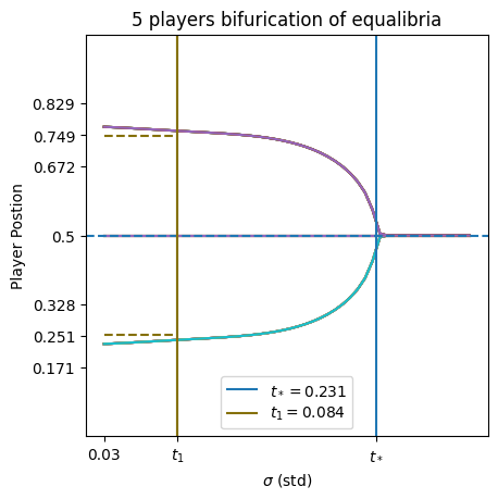
../../_images/bifurcation.png — This is a 5 player positions bifurcation plot for a 1d domain.#

the critical values are estimated via InflGame.domains.one_d.utils.critical_values_plot.

2d example

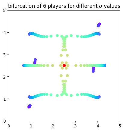
../../_images/2d_bifurcation.png — This is a 6 player positions bifurcation plot for a 2d domain.#

Simplex example

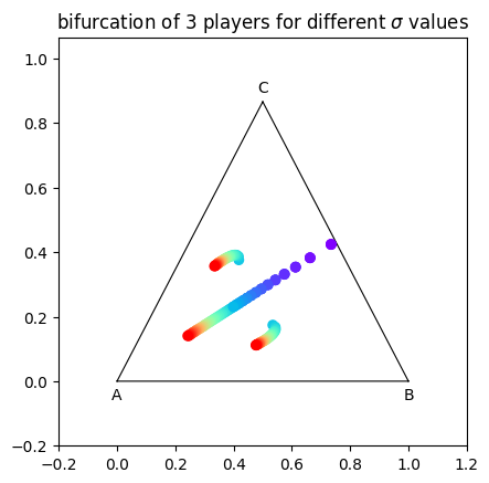
../../_images/simplex_bifurcation.png — This is a 3 player positions bifurcation plot for a simplex.#

Parameters:

matrixOptional[Dict]: Pre-computed matrix of final positions (optional, will compute if None).
reach_startfloat: Starting value of reach parameter.
reach_endfloat: Ending value of reach parameter.
reach_num_pointsint: Number of points in the reach parameter range.
time_stepsint: Number of gradient ascent steps.
initial_posUnion[List[float], np.ndarray]: Initial positions of agents.
current_alphafloat: Current alpha value.
toleranceOptional[float]: Tolerance for convergence.
tolerated_agentsOptional[int]: Number of agents allowed to tolerate deviations.
refinementsint: Refinement level for plotting.
plot_typestr: Type of plot (‘heat’, ‘trajectory’, etc.).
title_adsList[str]: Additional titles for the plot.
name_adsList[str]: Additional names for saved files.
savebool: Whether to save the plot.
save_typesList[str]: File types to save the plot.
return_matrixbool: Whether to return the final position matrix.
parallel_configsOptional[Dict[str, Union[bool, int]]]: Configuration dictionary for parallel processing with keys ‘parallel’, ‘max_workers’, ‘batch_size’.
cmapsdict: Color map configuration dictionary.
fontdict: Font configuration dictionary.
cbar_configdict: Colorbar configuration dictionary.
paper_figuredict: Paper figure configuration dictionary.
show_predbool: Whether to show predictions.
envelopebool: Whether to use envelope method.
optional_vlineOptional[List[float]]: Optional vertical lines to add to plot.
verbosebool: Whether to print verbose output.
completebool: Whether to compute complete bifurcation envelope.
learning_rateOptional[List]: Learning rate schedule.
percentageOptional[float]: Percentage threshold for envelope method.

Returns:

Union[torch.Tensor, matplotlib.figure.Figure]: The generated plot figure or final position matrix.

find_and_analyze_zero_crossings(test_eval, parameters_list, x_star=None, threshold=5.0)#

Complete workflow to find, refine, and analyze eigenvalue zero crossings.

Parameters:

test_evaltorch.Tensor: Tensor of eigenvalues.
parameters_listtorch.Tensor: Tensor of parameter values.
x_starOptional[torch.Tensor]: Theoretical critical point (if available).
thresholdfloat: Maximum absolute value to consider “close to zero”.

Returns:

Optional[dict]: Analysis results dictionary.

find_zero_crossings(test_eval, parameters_list, threshold=5.0)#

Identify parameter values where eigenvalue real parts are close to zero.

Parameters:

test_evaltorch.Tensor: Tensor of eigenvalues [n_params, n_agents].
parameters_listtorch.Tensor: Tensor of parameter values [n_params, n_agents].
thresholdfloat: Maximum absolute value to consider “close to zero”.

Returns:

Tuple[torch.Tensor, torch.Tensor, torch.Tensor]: Tuple of (parameter indices, parameter values, real parts) near zero crossings.

first_order_bifurcation_plot(processed_data, alpha_st=0, alpha_end=1, alpha_values=None, cutoff_index=None, title_ads=[], save=False, name_ads=[], font={'cbar_size': 16, 'default_size': 24, 'font_family': 'sans-serif', 'label_size': 10, 'legend_size': 12, 'table_size': 15, 'title_size': 34}, save_types=['.png', '.svg'], paper_figure={'figure_id': 'bif_diag', 'paper': False, 'section': '3_2_6'})#

Generate and plot first-order bifurcation diagram with stability analysis.

This method creates a visualization of first-order (saddle-node) bifurcations by computing equilibrium positions and their stability across a parameter range. The plot shows how equilibrium agent positions change as a resource parameter (alpha) varies, with stability indicated through InflGame.adaptive.jacobian.jacobian_stability_fast.

The method supports both original format (e.g., Gaussian kernels) and processed data format with pre-computed stability flips, making it flexible for different analysis workflows.

First-order bifurcations are characterized by the creation or annihilation of equilibrium pairs, typically visualized as branches that meet and disappear at critical parameter values.

Example Gaussian Bifurcation Diagram

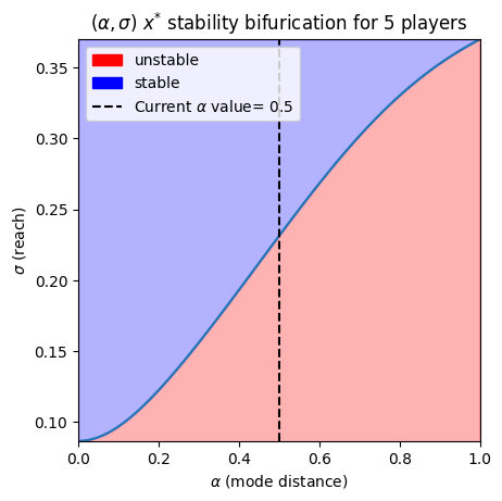
../../_images/first_order.png — First-order bifurcation plot for 5 players using symmetric Gaussian influence kernels.#

Parameters:

processed_datadict: Pre-processed bifurcation data with ‘unstable_flip’, ‘stable_flip’, and optionally ‘cycles_end’.
alpha_stfloat: Starting value of the resource parameter range.
alpha_endfloat: Ending value of the resource parameter range.
alpha_valuesOptional[np.ndarray]: Array of alpha (parameter) values corresponding to equilibria.
cutoff_indexOptional[int]: Index to truncate the data (useful for focusing on specific parameter ranges).
title_adsList[str]: Additional text to append to plot title.
savebool: Whether to save the plot to file.
name_adsList[str]: Additional text for saved filename.
fontDict: Font configuration dictionary with keys: ‘default_size’, ‘cbar_size’, ‘title_size’, ‘legend_size’, ‘table_size’, ‘label_size’, ‘font_family’.
save_typesList[str]: List of file formats for saving (e.g., [‘.png’, ‘.svg’]).
paper_figuredict: Configuration for paper figure saving with keys: ‘paper’ (bool), ‘section’ (str), ‘figure_id’ (str).

Returns:

matplotlib.figure.Figure: The generated matplotlib figure object.

Examples

fig = vis.first_order_bifurcation_plot(
    processed_data=processed,
    alpha_st=0.0,
    alpha_end=1.0,
    save=True,
    name_ads=['my_bifurcation'],
    title_ads=['3-Player System']
)
fig.show()

first_order_bifurcation_plot_old(agent_parameter_instance, resource_distribution_type, resource_entropy=False, infl_entropy=False, alpha_current=0.5, alpha_st=0, alpha_end=1, varying_parameter_type='mean', fixed_parameters_lst=None, name_ads=[], title_ads=[], save_types=['.png', '.svg'], paper_figure={'figure_id': 'first_order_bifurcation_plot', 'paper': False, 'section': 'A'}, font={'cbar_size': 16, 'default_size': 15, 'font_family': 'sans-serif', 'legend_size': 12, 'title_size': 18})#

Plots the first-order bifurcation for agents over a range of alpha values (resource parameters) via func:jacobian_stability_fast. Currently only works for Gaussian influence and multi-variate Gaussian influence kernels.

Gaussian example

Parameters:

agent_parameter_instanceUnion[List[float], np.ndarray]: Parameters for the influence function.
resource_distribution_typestr: Type of resource distribution.
resource_entropybool: Whether to calculate resource entropy.
infl_entropybool: Whether to calculate influence entropy.
alpha_currentfloat: Current alpha value.
alpha_stfloat: Starting value of alpha.
alpha_endfloat: Ending value of alpha.
varying_parameter_typestr: Type of varying parameter (e.g., ‘mean’).
fixed_parameters_lstOptional[List[float]]: List of fixed parameters.
name_adsList[str]: Additional names for saved files.
title_adsList[str]: Additional titles for the plot.
save_typesList[str]: File types to save the plot.

Returns:

matplotlib.figure.Figure: The generated plot figure.

generate_combined_figure(alpha, test_processed, results_list, search, figsize=(32, 22), width_ratios=[1, 1], height_ratios=[1, 1, 1], hspace=0.4, wspace=0.12, region_labels=['a', 'b', 'c', 'd'], save=False, save_types=['.png', '.svg'], paper_figure={'figure_id': 'fig_combined', 'paper': True, 'section': '3_2_6'}, font={'cbar_size': 16, 'default_size': 32, 'font_family': 'sans-serif', 'legend_size': 12, 'title_size': 40})#

Generate the standardized combined bifurcation and equilibrium analysis figure.

Delegates to InflGame.domains.one_d.one_plots.generate_combined_bifurcation_figure.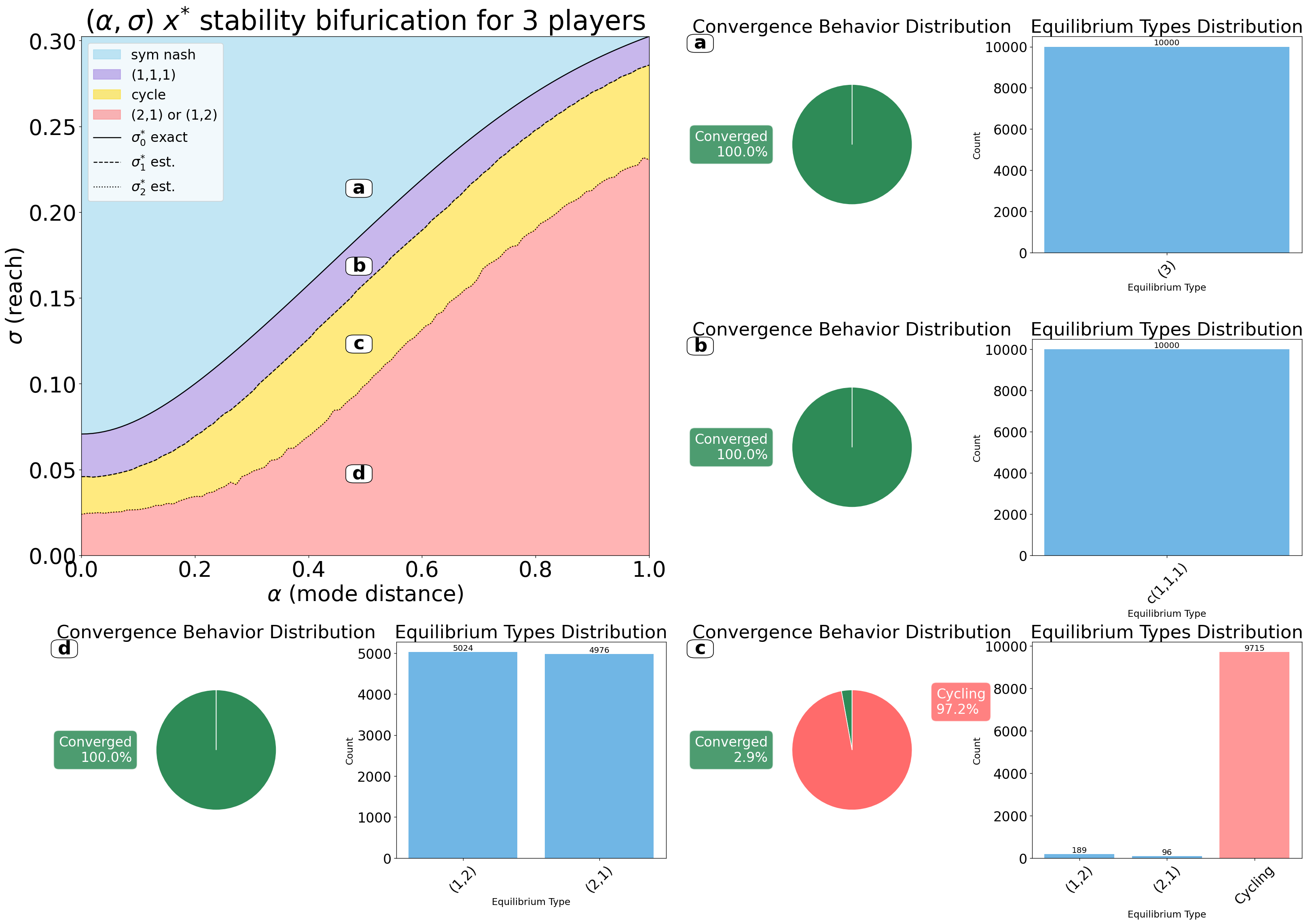

../../_images/combined_figure.png — Combined first-order bifurcation diagram with regional equilibrium panels.#

Parameters:

alphaarray-like: Alpha (resource) parameter values for the bifurcation sweep.
test_processeddict: Pre-processed bifurcation data (output of the bifurcation pipeline).
results_listList[dict]: Exactly four region result dicts [results1, results2, results3, results4].
searchsearch_env: Configured monte_search.search_env instance used to render equilibrium panels.
figsizeTuple[float, float]: Figure size in inches (width, height).
width_ratiosList[float]: Column width ratios for the 3×2 GridSpec layout.
height_ratiosList[float]: Row height ratios for the 3×2 GridSpec layout.
hspacefloat: Vertical spacing between subplot rows.
wspacefloat: Horizontal spacing between subplot columns.
region_labelsList[str]: Labels placed on both the bifurcation diagram and the panel headers.
savebool: Whether to save the figure to disk.
save_typesList[str]: File extensions used when saving.
paper_figuredict: Paper metadata: {'paper': bool, 'section': str, 'figure_id': str}.
fontdict: Font configuration: {'default_size', 'cbar_size', 'title_size', 'legend_size', 'font_family'}.

Returns:

matplotlib.figure.Figure

grad_plot(title_ads=[], save=False, name_ads=[], font={'cbar_size': 16, 'default_size': 15, 'font_family': 'sans-serif', 'legend_size': 12, 'title_size': 18}, save_types=['.png', '.svg'], paper_figure={'figure_id': 'grad_plot', 'paper': False, 'section': 'A'})#

Plots the gradients of agents as the lines versus time.

\[\frac{\partial}{\partial x_{(i,l)}}u_i(x)=\sum_{k=1}^{K}G_{i,k}(x_i,b_k)\frac{\partial}{\partial x_{(i,l)}}ln(f_{i}(x_i,b_k))\]

Where \(x_i\) is the \(i\) th players position, \(b_k\in \mathbb{B}\) are the bin/resource points, \(B(b_k)\) is the resource value at \(b_k\), and \(G_i(x_i,b_k)\) probability of player \(i\) influencing the bin point \(b\). The gradients are calculated via InflGame.adaptive.grad_func_env.gradient.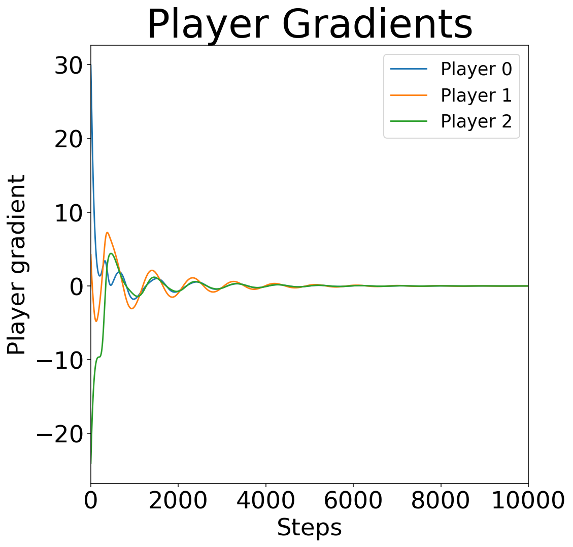

../../_images/gradient.png — Example gradient trajectories for a three-player game in a 1D domain.#

Parameters:

title_adsList[str]: Additional titles for the plot.
savebool: Whether to save the plot.
name_adsList[str]: Additional names for saved files.
save_typesList[str]: File types to save the plot.

Returns:

matplotlib.figure.Figure: The generated plot figure.

jacobian_stability_fast(agent_parameter_instance, resource_distribution_type, resource_parameters, resource_entropy=False, infl_entropy=False)#

Calculate the stability of the symmetric Nash equilibrium via analytical computation of maximum eigenvalues.

This method analytically computes the Jacobian matrix eigenvalues at the symmetric Nash equilibrium to determine stability regions. Currently supports Gaussian and multi-variate Gaussian influence kernels.

The symmetric Nash equilibrium position is computed based on the resource distribution, and stability is assessed by examining the sign of the maximum real eigenvalue of the Jacobian.

Parameters:

agent_parameter_instanceUnion[List[float], np.ndarray]: Parameters for the influence function (e.g., sigma for Gaussian).
resource_distribution_typestr: Type of resource distribution (‘gauss_mix_2m’, ‘uniform’, etc.).
resource_parametersUnion[List[float], np.ndarray]: Parameters defining the resource distribution for each test point.
resource_entropybool: Whether to calculate and return entropy of resource distributions.
infl_entropybool: Whether to calculate and return entropy of influence distributions.

Returns:

Tuple[List[torch.Tensor], List[float], List[float]]: Tuple containing: - List of critical parameter values (one per resource configuration) - List of resource entropies (empty if resource_entropy=False) - List of influence entropies (empty if infl_entropy=False)

Raises:

ValueError: If influence type is not ‘gaussian’ or ‘multi_gaussian’.

node_to_images(main, left_matrices, right_matrices, reach_parameters, reach_start, reach_end, key_tolerance=2, box_width=0.05, space=None, title_ads=[], font={'cbar_size': 12, 'default_size': 24, 'font_family': 'sans-serif', 'label_size': 24, 'legend_size': 12, 'title_size': 64}, hide_text=False, max_reward=None, show_column_labels=True)#

process all matrices and create images for each node

Parameters:

maindict: Main bifurcation matrix
left_matriceslist: List of left branch matrices
right_matriceslist: List of right branch matrices
reach_parameterstorch.Tensor: Reach parameters
key_toleranceint: Minimum distance between keys to process. If next key is closer than this, skip current key.

plot_equilibrium_heatmap(newton_search_data, title_ads=[], save=False, name_ads=[], font={'cbar_size': 16, 'default_size': 15, 'font_family': 'sans-serif', 'label_size': 10, 'legend_size': 12, 'table_size': 15, 'title_size': 18}, save_types=['.png', '.svg'], paper_figure={'figure_id': 'equil_heat', 'paper': False, 'section': '3_2_6'})#

Generate and plot a heatmap of equilibrium positions in a 1D influence game. This method visualizes the equilibrium positions of agents in a 1D influence game as a heatmap, with optional stability analysis overlay.

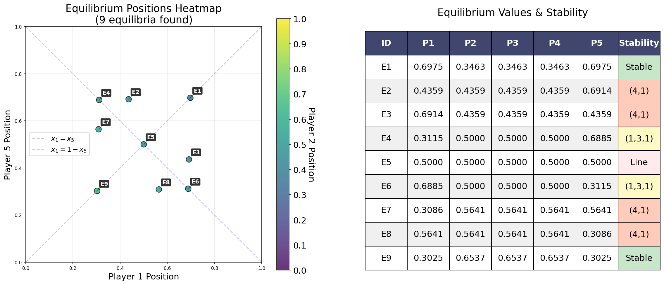
../../_images/equilibrium_heatmap.png — Example equilibrium heatmap from a Newton grid search.#

Parameters:

newton_search_datadict | list | np.ndarray: Equilibrium search results used to build the heatmap.
title_adsList[str]: Additional text to append to plot title.
savebool: Whether to save the plot to file.
name_adsList[str]: Additional text for saved filename.
fontDict: Font configuration dictionary with keys ‘default_size’, ‘cbar_size’, ‘title_size’, ‘legend_size’, ‘table_size’, ‘label_size’, ‘font_family’.
save_typesList[str]: List of file formats for saving (e.g., [‘.png’, ‘.svg’]).
paper_figuredict: Configuration for paper figure saving with keys: ‘paper’ (bool), ‘section’ (str), ‘figure_id’ (str).

Returns:

matplotlib.figure.Figure: The generated matplotlib figure object.

pos_plot(title_ads=[], fig_size=(18, 18), save=False, name_ads=[], line_thickness=2, font={'cbar_size': 16, 'default_size': 15, 'font_family': 'sans-serif', 'legend_size': 12, 'title_size': 18}, save_types=['.png', '.svg'], paper_figure={'figure_id': 'pos_plot', 'paper': False, 'section': 'A'}, svg_options=None)#

Plots the positions of agents over gradient ascent steps. The positions of players are calculated via the results of InflGame.adaptive.grad_func_env.gradient_ascent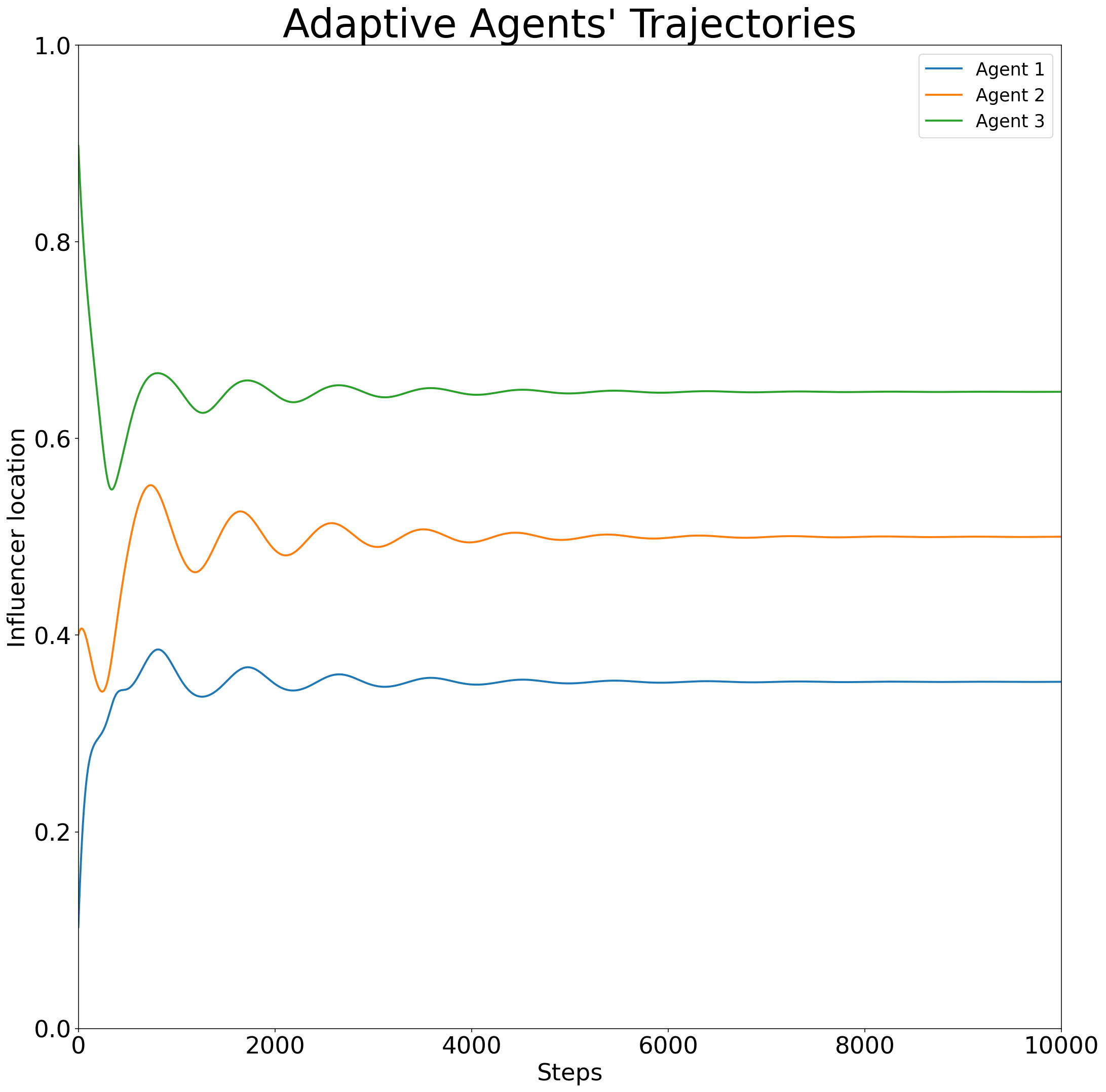

../../_images/pos_plot.png — Example trajectory of agent positions over gradient-ascent steps in a 1D domain.#

Parameters:

title_adsList[str]: Additional titles for the plot.
savebool: Whether to save the plot.
name_adsList[str]: Additional names for saved files.
save_typesList[str]: File types to save the plot.

Returns:

matplotlib.figure.Figure: The generated plot figure.

position_at_equalibirum_histogram(reach_parameter=0.5, time_steps=100, initial_pos=0, current_alpha=0.5, tolerance=None, tolerated_agents=None, title_ads=[], name_ads=[], save=False, save_types=['.png', '.svg'], return_pos=False, parallel=True, max_workers=None, batch_size=None, paper_figure={'figure_id': 'position_at_equalibirum_histogram', 'paper': False, 'section': 'A'}, font={'cbar_size': 16, 'default_size': 15, 'font_family': 'sans-serif', 'legend_size': 12, 'title_size': 18})#

Plot the histogram of agents’ positions at equilibrium for a given reach parameter via the function InflGame.adaptive.grad_func_env.gradient_ascent . This only works for ‘1d’ domains.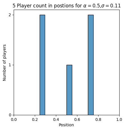

../../_images/histogram.png — This is the histogram of player positions at equilibrium for 5 player game.#

Parameters:

reach_parameterfloat: Reach parameter value.
time_stepsint: Number of gradient ascent steps.
initial_posUnion[List[float], np.ndarray]: Initial positions of agents.
current_alphafloat: Current alpha value.
toleranceOptional[float]: Tolerance for convergence.
tolerated_agentsOptional[int]: Number of agents allowed to tolerate deviations.
title_adsList[str]: Additional titles for the plot.
name_adsList[str]: Additional names for saved files.
savebool: Whether to save the plot.
save_typesList[str]: File types to save the plot.
return_posbool: Whether to return the final positions.
parallelbool: Whether to use parallel processing.
max_workersOptional[int]: Maximum number of parallel workers (defaults to CPU count).
batch_sizeOptional[int]: Batch size for processing (auto-calculated if None).
paper_figuredict: Paper figure configuration dictionary.
fontdict: Font configuration dictionary.

Returns:

Union[matplotlib.figure.Figure, Tuple[matplotlib.figure.Figure, np.ndarray]]: The generated plot figure or final positions.

prob_plot(position=[], parameters=[], title_ads=[], save=False, name_ads=[], font={'cbar_size': 16, 'default_size': 15, 'font_family': 'sans-serif', 'legend_size': 12, 'title_size': 18}, save_types=['.png', '.svg'], paper_figure={'figure_id': 'prob_plot', 'paper': False, 'section': 'A'})#

Plot the probability distribution of agents’ influence over a bin/resource point via their relative influence over that point

\[G_{i,k}(\mathbf{x},b_k)=\frac{f_{i}(x_i,b_k)}{\sum_{j=1}^{N}f_{j}(x_j,b_k)}.\]

where \(f_{i}(x_i,b_k)\) is the \(i\) th players influence. The probabilities are calculated via InflGame.adaptive.grad_func_env.prob_matrix .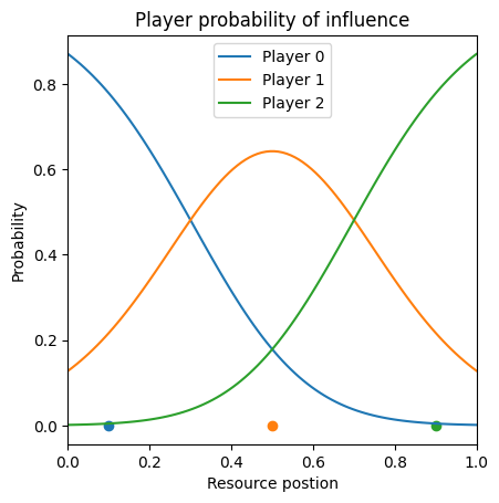

../../_images/probability.png — This is an example of the a three player game with agents in position \([.1,.45,.9]\) . Here the the influence kernels are symmetric gaussian with with parameter (reach) \(\sigma=0.25\) .#

There can is also the option to have a fixed third party (infl_csift==True) and/or abstaining voters if (infl_fshift==True).

Parameters:

positionnp.ndarray: Positions of agents.
parametersnp.ndarray: Parameters for the influence function.
title_adsList[str]: Additional titles for the plot.
savebool: Whether to save the plot.
name_adsList[str]: Additional names for saved files.
save_typesList[str]: File types to save the plot.

Returns:

matplotlib.figure.Figure: The generated plot figure.

resource_distribution_plot(alpha=None, show_alpha_line=True, title='Resource distribution', fig_size=(12, 8), line_width=2, save=False, name_ads=[], save_types=['.png', '.svg'], paper_figure={'figure_id': 'resource_dist', 'paper': False, 'section': 'A'}, font={'alpha_size': 20, 'cbar_size': 16, 'default_size': 15, 'font_family': 'sans-serif', 'legend_size': 12, 'title_size': 18}, y_padding=1.25)#

Plots the resource distribution with optional alpha line annotation for bimodal distributions.

For bimodal Gaussian distributions, this function draws a dashed line between the two peaks and labels it with \(\alpha\), representing the separation distance between peaks. The peak positions are calculated as \(0.5 - \alpha/2\) and \(0.5 + \alpha/2\).

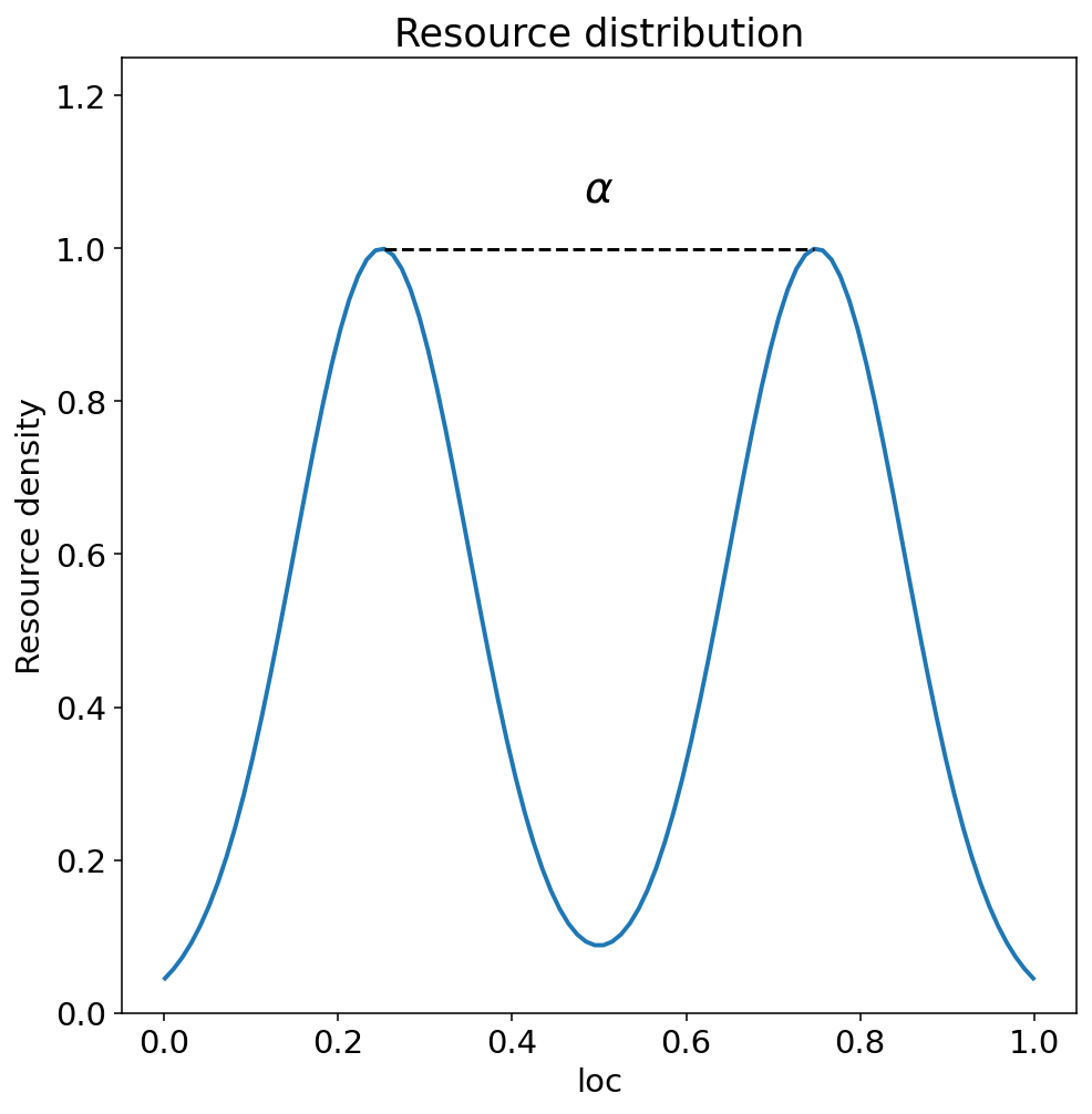
../../_images/resource_distribution.png — Example bimodal resource distribution with an \(\alpha\) annotation.#

Parameters:

alphafloat, optional: The separation parameter for bimodal distributions. If provided, a dashed line will be drawn between the peaks at positions (0.5 - alpha/2) and (0.5 + alpha/2).
show_alpha_linebool: Whether to show the alpha annotation line between peaks.
titlestr: Title for the plot.
fig_sizeTuple: Figure size as (width, height).
line_widthfloat: Width of the distribution line.
savebool: Whether to save the plot.
name_adsList[str]: Additional names for saved files.
save_typesList[str]: File types to save the plot.
paper_figuredict: Configuration for paper figure saving.
fontdict: Font configuration dictionary.
y_paddingfloat: Multiplier for y-axis upper limit to add space for labels.

Returns:

matplotlib.figure.Figure: The generated plot figure.

Examples

# Plot bimodal distribution with alpha annotation
fig = shell.resource_distribution_plot(alpha=0.5, show_alpha_line=True)

reward_groups_stacked(idx=0, rwd_type='bifurication', max_reward=None, box_width=0.01, matrix=None, space=None, title_ads=[], save=False, name_ads=[], reach_start=0.03, reach_end=0.3, reach_num_points=200, font={'cbar_size': 16, 'default_size': 15, 'font_family': 'sans-serif', 'label_size': 10, 'legend_size': 12, 'table_size': 15, 'title_size': 18}, show_outline=True, show_total_outline=True, show_label_box=True, aspect=1, save_types=['.png', '.svg'], paper_figure={'figure_id': 'reward_groups_stacked', 'paper': False, 'section': '3_2_6'})#: Plot stacked reward groups across agents for a selected bifurcation slice.

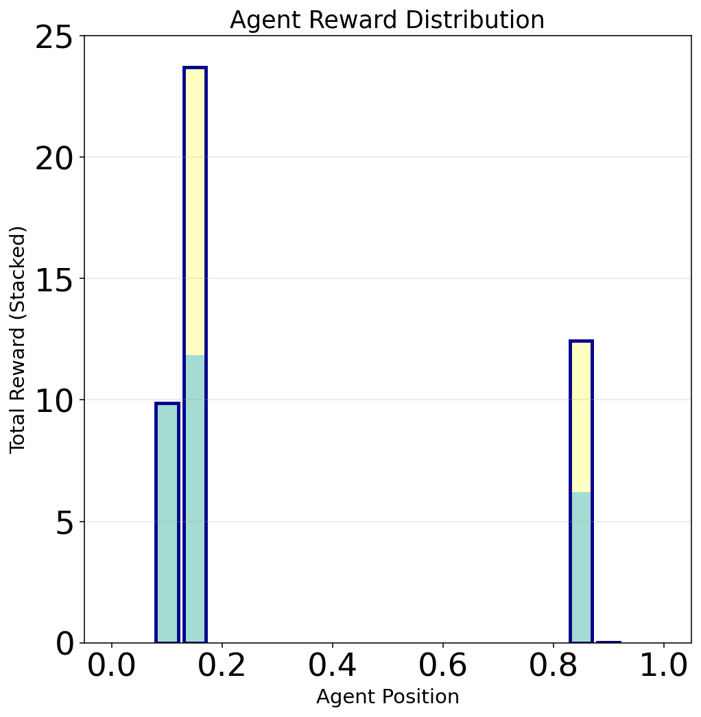
Stacked reward groups at a fixed reach for a five-player bifurcation.#

setup_adaptive_env()#

Set up the adaptive environment for the simulation.

This initializes the InflGame.adaptive.grad_func_env.AdaptiveEnv instance with all parameters configured in the Shell constructor. The adaptive environment handles gradient ascent computation, influence calculations, and trajectory tracking.

After calling this method, gradient ascent can be performed via self.field.gradient_ascent() and results accessed through self.field.pos_matrix and self.field.grad_matrix.

setup_bifurcation_env()#

Set up the bifurcation environment for parameter sweep analysis.

This initializes the InflGame.adaptive.bifurcation_analysis.BifurcationEnv instance for computing equilibrium positions across parameter ranges. The bifurcation environment extends the adaptive environment with specialized methods for systematic parameter variation.

After calling this method, bifurcation analysis can be performed via methods like self.bif_field.final_pos_over_reach() and self.bif_field.equilibrium_bifurcation_complete().

simple_diagonal_test_point(point=None)#

Test a single point to verify gradient ascent functionality.

This diagnostic method performs a simple gradient ascent run from a specified starting point to verify that the core optimization loop is working correctly. Useful for debugging and validation.

Parameters:

pointOptional[torch.Tensor]: Starting position for agents (defaults to [0.3, 0.5, 0.7] if None).

Returns:

bool: True if gradient ascent successfully generated a path, False otherwise.

three_agent_pos_3A1d(x_star=None, title_ads=[], save=False, name_ads=[], line_thickness=2.0, fontL={'cbar_size': 16, 'default_size': 15, 'font_family': 'sans-serif', 'legend_size': 12, 'title_size': 18}, fontR={'cbar_size': 16, 'default_size': 15, 'font_family': 'sans-serif', 'legend_size': 12, 'title_size': 18}, fontmain={'cbar_size': 16, 'default_size': 15, 'font_family': 'sans-serif', 'legend_size': 12, 'title_size': 18}, save_types=['.png', '.svg'], paper_figure={'figure_id': 'pos_plot', 'paper': False, 'section': 'A'}, limits_params={'tick_count_left': 5, 'tick_count_right': 5, 'xlim_left': None, 'xlim_right': None})#

Create combined visualization showing three-agent dynamics in 3D space alongside position trajectories.

This method produces a side-by-side comparison plot for three-player games in 1D domains: - Left panel: 3D visualization of agent positions over time - Right panel: Traditional position vs. time plot

Only available for 1D domains with exactly 3 agents, as it visualizes the 3-dimensional trajectory space where each axis represents one agent’s position.

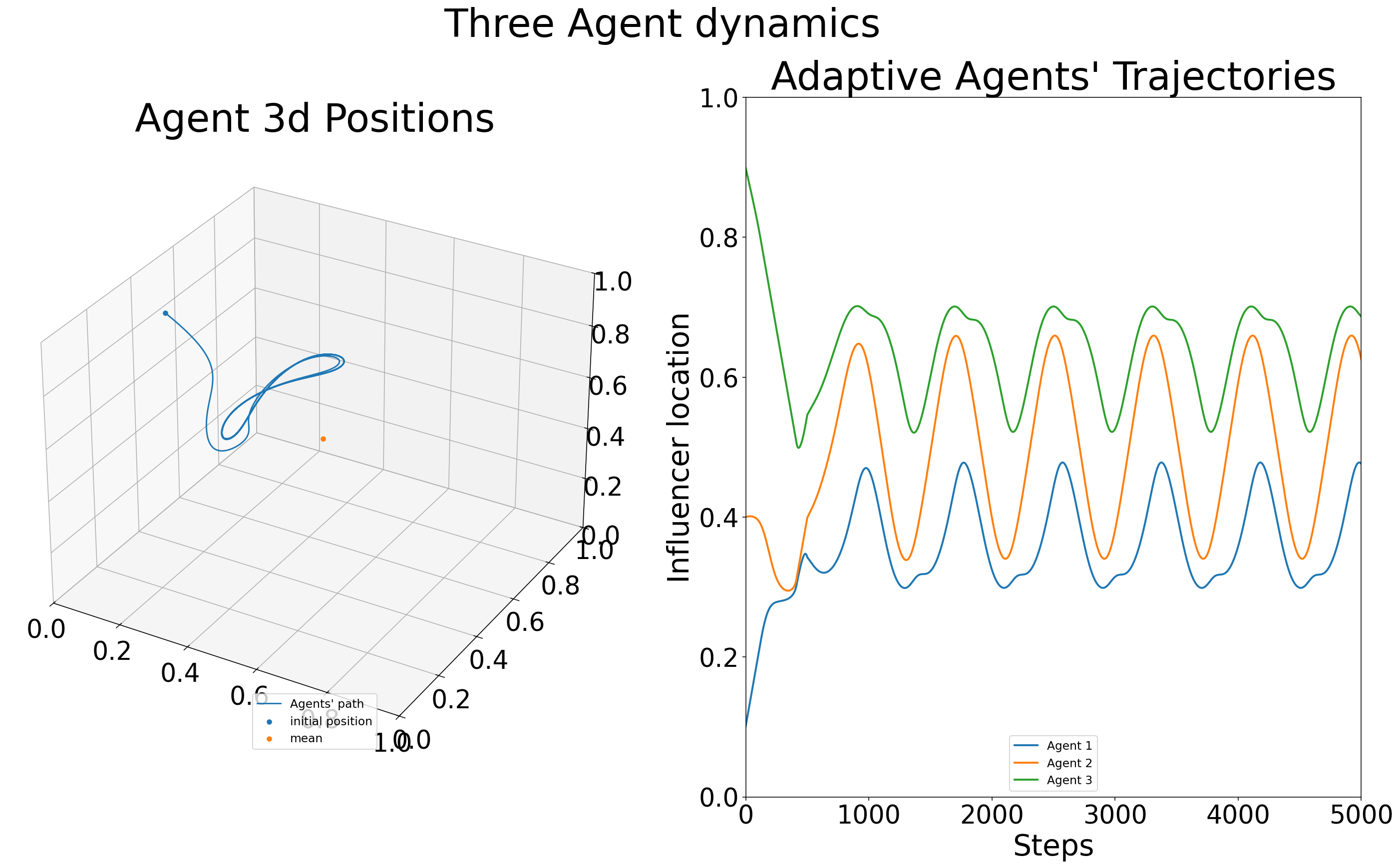
../../_images/three_agent_pos_3A1d.png — Side-by-side 3D position path and time-series trajectories for three agents.#

Parameters:

x_starOptional[float]: Equilibrium position (computed from resource distribution if not provided).
title_adsList[str]: Additional title text components.
savebool: Whether to save the figure to file.
name_adsList[str]: Additional filename components for saving.
fontLdict: Font configuration dictionary for left (3D) panel.
fontRdict: Font configuration dictionary for right (position) panel.
fontmaindict: Font configuration dictionary for main title.
save_typesList[str]: File formats for saving (e.g., [‘.png’, ‘.svg’]).
paper_figuredict: Paper figure configuration with ‘paper’, ‘section’, ‘figure_id’ keys.

Returns:

matplotlib.figure.Figure: Combined matplotlib figure with both visualizations.

Raises:

ValueError: If domain_type is not ‘1d’ or num_agents is not 3.

three_agent_pos_3d(x_star=None, title_ads=[], name_ads=[], save=False, font={'cbar_size': 16, 'default_size': 15, 'font_family': 'sans-serif', 'legend_size': 12, 'title_size': 18}, save_types=['.png', '.svg'], paper_figure={'figure_id': 'three_players', 'paper': False, 'section': 'A'})#

Visualize dynamics for three players: demonstrates the players positions changing in time in 3-d space. Demonstrating the instability of 3-players in influencer games. Given that this function is in 3-d space for players with 1-d strategies there isn’t a way to visualize the 3 player dynamics in games with more then 1d strategy spaces. The positions of players are calculated via the results of InflGame.adaptive.grad_func_env.gradient_ascent .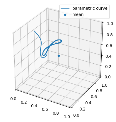

../../_images/three_player.png — This is an example of the three player dynamics via their positions in time`.#

Parameters:

x_starOptional[float]: Equilibrium position.
title_adsList[str]: Additional titles for the plot.
name_adsList[str]: Additional names for saved files.
savebool: Whether to save the plot.
save_typesList[str]: File types to save the plot.

Returns:

matplotlib.figure.Figure: The generated plot figure.

threed_fixed_diagonal_view(resolution=5, time_steps=10000, show_planes=True, figsize=(12, 10), seed=42, include_boundaries=True, elev=10, azim=45, num_workers=4, use_parallel=True, only_results=False, verbose=False)#

Creates a 3D plot with fixed view looking down the x=y=z diagonal line, showing gradient ascent trajectories from multiple starting points with optional parallel processing.

This method visualizes how agents starting from different initial positions converge or diverge under gradient ascent dynamics. The view is oriented to look down the main diagonal (x=y=z line) to better visualize symmetric and asymmetric equilibria. Paths are color-coded by the ordering of initial agent positions.

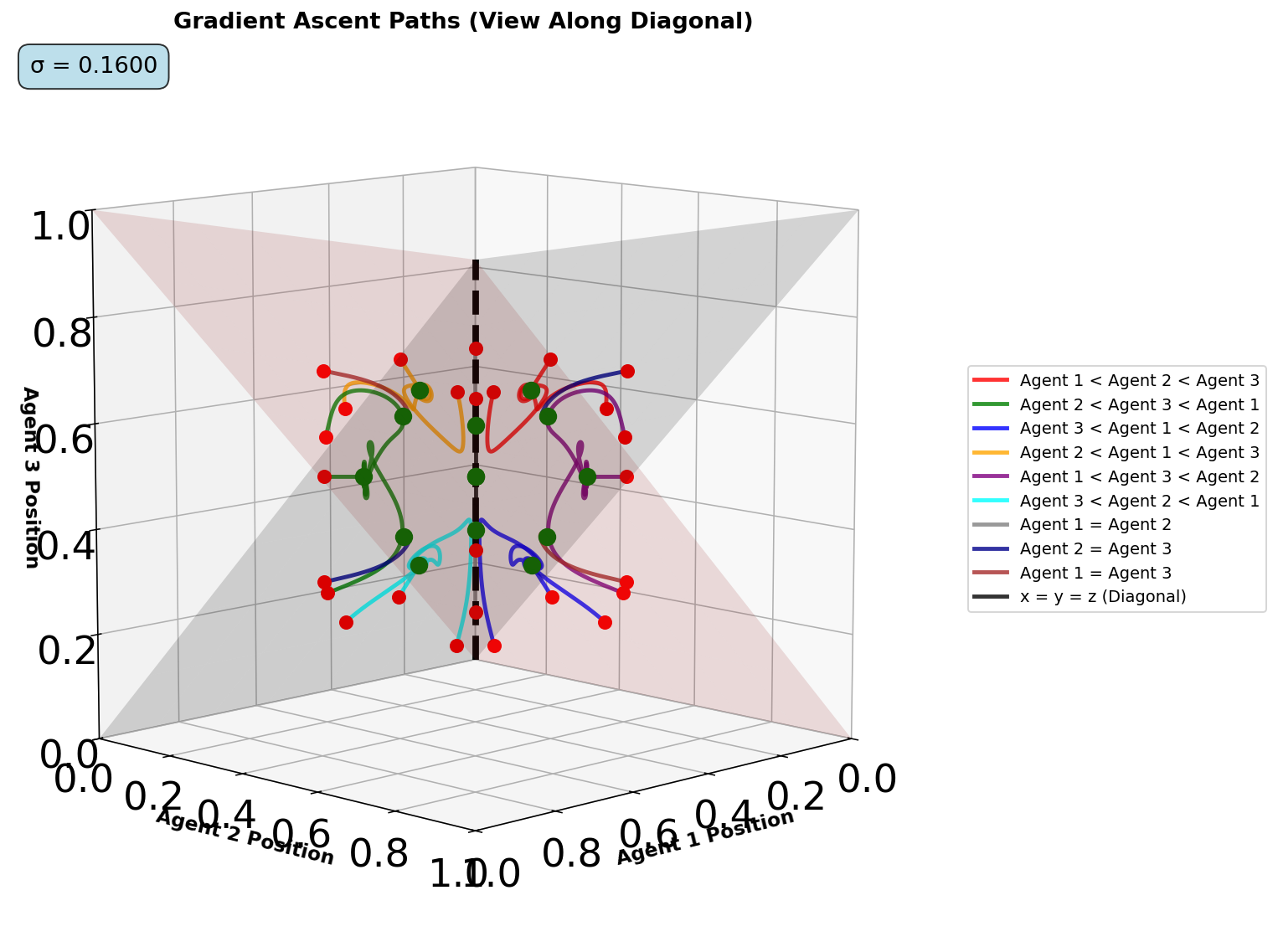
../../_images/threed_fixed_diagonal_view.png — Diagonal-view 3D trajectories from multiple initial conditions.#

Parameters:

resolutionint: Number of test points per dimension (total points = resolution^3).
time_stepsint: Maximum gradient ascent iterations per trajectory.
show_planesbool: Whether to display equality planes (x=y, y=z, x=z) for reference.
figsizeTuple[int, int]: Figure dimensions in inches (width, height).
seedint: Random seed for reproducibility of starting points.
include_boundariesbool: Whether to include boundary points in the analysis.
elevint: Elevation viewing angle in degrees (lower values look more downward).
azimint: Azimuth viewing angle in degrees (rotation around vertical axis).
num_workersint: Number of parallel worker processes.
use_parallelbool: Whether to use parallel processing for trajectory computation.
only_resultsbool: If True, return only the results dictionary without creating plot.
verbosebool: Whether to print detailed progress information.

Returns:

Tuple[matplotlib.figure.Figure, List[dict]]: Tuple of (matplotlib figure, list of trajectory result dictionaries).

threed_fixed_diagonal_view_gif(max_frames, output_filename='3d_diagonal_traces.gif', resolution=5, time_steps=10000, show_planes=True, figsize=(12, 10), seed=42, include_boundaries=True, elev=10, azim=45, num_workers=4, use_parallel=True, reach_start=0.08, reach_end=0.25, optimize_memory=True, dpi=100, fps=10, quality=8, verbose=False)#

Create a 3D diagonal view GIF showing gradient ascent traces over varying reach parameters. Similar to dist_pos_gif but for 3D visualization. Works by varying the reach parameters and creating frames of threed_fixed_diagonal_view .

../../_images/threed_fixed_diagonal_view.gif — Animated diagonal-view trajectories as the reach parameter varies.#

Optimized Performance Features: - Direct memory writing without intermediate files - Matplotlib figure recycling for memory efficiency - Optimized frame sampling - Configurable quality vs speed trade-offs

Parameters:

max_framesint: Maximum number of frames for the gif.
output_filenamestr: Name of the output GIF file.
resolutionint: Resolution for point sampling in 3D plot.
time_stepsint: Number of gradient ascent steps.
show_planesbool: Whether to show equality planes in 3D plot.
figsizetuple: Figure size for each frame.
seedint: Random seed for reproducibility.
include_boundariesbool: Whether to include boundary points in 3D plot.
elevint: Elevation angle for 3D view.
azimint: Azimuth angle for 3D view.
num_workersint: Number of parallel workers for 3D processing.
use_parallelbool: Whether to use parallel processing for 3D plots.
reach_startfloat: Starting reach parameter value.
reach_endfloat: Ending reach parameter value.
optimize_memorybool: Whether to use memory optimization techniques.
dpiint: DPI for the frames (lower = faster, higher = better quality).
fpsint: Frames per second for the GIF.
qualityint: GIF compression quality (1-10, lower = smaller file).
verbosebool: Whether to print progress information.

Returns:

matplotlib.figure.Figure: The final frame figure for display.

threed_gradient_ascent_paths_interactive(resolution=5, time_steps=10000, start_color='red', end_color='green', title='3D Path of Gradient Ascent (Interactive)', show_planes=False)#

Creates an interactive 3D plot of gradient ascent paths from multiple starting points, with paths color-coded based on the initial position’s quadrant.

The docs embed is a live Plotly figure (zoom / pan / hover). It is generated into docs/_static/plotly/ and isolated from the Sphinx theme via an iframe.

Parameters:

resolutionint: Resolution of the cube grid (points per dimension).
time_stepsint: Maximum number of steps for gradient ascent.
start_colorstr: Color of the starting points.
end_colorstr: Color of the ending points (for converged paths).
titlestr: Plot title.
show_planesbool: Whether to show the equality planes (x=y, y=z, z=x).

Returns:

plotly.graph_objects.Figure: Interactive 3D plot.

vect_plot(agent_id=None, parameter_instance=None, cmap='viridis', typelabels=['A', 'B', 'C'], ids=[0, 1], pos=None, title_ads=[], save=False, name_ads=[], save_types=['.png', '.svg'], paper_figure={'figure_id': 'vect_plot', 'paper': False, 'section': 'A'}, font={'cbar_size': 16, 'default_size': 15, 'font_family': 'sans-serif', 'legend_size': 12, 'title_size': 18}, alt_form=False, **kwargs)#

Plot the vector field of gradients for a specific agents calculated by the function calc_direction_and_strength . Currently only supports 1d domains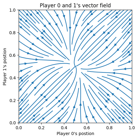

../../_images/vector_field.png — This is an example of the vector field for a three player game with only players 1 and 2 dynamics shown (player 3 is fixed)`.#

Parameters:

agent_idint: ID of the agent.
parameter_instanceUnion[List[float], np.ndarray, torch.Tensor]: Parameters for the influence function.
cmapstr: Colormap for the plot.
typelabelsList[str]: Labels for agent types.
idsList[int]: IDs of agents of interest.
posOptional[torch.Tensor]: Positions of agents.
title_adsList[str]: Additional titles for the plot.
savebool: Whether to save the plot.
name_adsList[str]: Additional names for saved files.
save_typesList[str]: File types to save the plot.
kwargs: Additional arguments for plotting.

Returns:

matplotlib.figure.Figure: The generated plot figure.