Bifurcation Analysis#
Bifurcation Analysis Module#
This module provides comprehensive bifurcation analysis tools for studying equilibrium dynamics, stability transitions, and parameter-dependent behaviors in adaptive environments for influencer games. It includes methods for computing equilibrium positions across parameter ranges, detecting bifurcation points, and analyzing stability properties.
The module is designed to work with the AdaptiveEnv class and provides a framework for understanding how agent behaviors and equilibrium configurations change as system parameters vary.
Dependencies:#
InflGame.adaptive.grad_func_env
InflGame.adaptive.jacobian
InflGame.utils
InflGame.kernels
InflGame.domains
Usage:#
The BifurcationEnv class can be used to analyze bifurcations and equilibrium dynamics in simulations performed using the AdaptiveEnv class. It supports various analysis types, including equilibrium bifurcation diagrams, stability analysis, and multi-order bifurcation detection.
Examples#
from InflGame.adaptive.bifurcation_analysis import BifurcationEnv
import torch
import numpy as np

# Initialize the BifurcationEnv
bif_env = BifurcationEnv(
    num_agents=3,
    agents_pos=np.array([0.2, 0.5, 0.8]),
    parameters=torch.tensor([1.0, 1.0, 1.0]),
    resource_distribution=torch.tensor([10.0, 20.0, 30.0]),
    bin_points=np.array([0.1, 0.4, 0.7]),
    infl_configs={'infl_type': 'gaussian'},
    learning_rate_type='cosine_annealing',
    learning_rate=[0.0001, 0.01, 15],
    time_steps=100,
    domain_type='1d',
    domain_bounds=[0, 1]
)

# Set up the adaptive environment
bif_env.setup_adaptive_env()

# Compute equilibrium bifurcation diagram
equilibria = bif_env.equilibrium_bifurcation_complete(
    reach_start=0.1,
    reach_end=1.0,
    reach_num_points=50
)
Classes
- class InflGame.adaptive.bifurcation_analysis.BifurcationEnv(num_agents, agents_pos, parameters, resource_distribution, bin_points, infl_configs={'infl_type': 'gaussian'}, learning_rate_type='cosine_annealing', learning_rate=[0.0001, 0.01, 15], time_steps=100, fp=0, infl_cshift=False, cshift=None, infl_fshift=False, Q=None, domain_type='1d', domain_bounds=[0, 1], resource_type='na', domain_refinement=10, tolerance=1e-05, tolerated_agents=None, ignore_zero_infl=False, device=None)#
Bifurcation analysis environment for studying equilibrium dynamics and stability transitions.
The BifurcationEnv class provides a comprehensive framework for analyzing bifurcation phenomena in adaptive dynamics across various domains (1D, 2D, and simplex). It supports computing equilibrium positions over parameter ranges, detecting bifurcation points of multiple orders, and analyzing stability properties through Jacobian analysis.
This class is designed to work in conjunction with the AdaptiveEnv class and provides specialized methods for understanding how system behavior changes as parameters vary, including identifying critical parameter values where qualitative changes in dynamics occur.
Methods
Compute complete equilibrium bifurcation diagram over a parameter range.
final_pos_over_reach(reach_parameters, ...)Calculate final equilibrium positions of agents over a range of reach parameters.
final_pos_over_reach_envelope(...[, ...])Calculate the envelope of equilibrium positions over a parameter range.
find_convergence_intersections(reach_parameters)Find parameter values where agent positions converge across different position variants.
find_second_order_bifs(bin_points, ...[, ...])Detect second-order (pitchfork or transcritical) bifurcation points.
find_third_order_bifurcations_refined(...[, ...])Detect third-order (subcritical or supercritical) bifurcation points with iterative refinement.
first_order_bifurcation_plot(processed_data)Generate and plot first-order bifurcation diagram with stability analysis.
learning_rate_large_end(resource_parameter)Determine appropriate learning rate upper bound for bifurcation analysis.
Set up the adaptive environment for bifurcation analysis.
- equilibrium_bifurcation_complete(reach_start=0.03, reach_end=0.3, reach_num_points=30, time_steps=100, initial_pos=None, tolerance=None, tolerated_agents=None, parallel_configs=None, envelope=False, verbose=True)#
Compute complete equilibrium bifurcation diagram over a parameter range.
This method generates a comprehensive bifurcation diagram by computing equilibrium positions across a range of reach parameter values, testing multiple initial position configurations to capture all stable equilibria. This is the primary method for creating bifurcation diagrams that visualize how equilibrium configurations change as parameters vary.
Key Features:
Proper state management with restoration after computation
Memory efficient matrix clearing between computations
Parameter validation and sensible defaults
Support for both single and envelope (max/min) equilibria
Optimized position generation for exploring initial condition space
Parallel processing support for large parameter sweeps
- Parameters:
- reach_startfloat
Starting value of reach parameter range.
- reach_endfloat
Ending value of reach parameter range.
- reach_num_pointsint
Number of parameter values to sample in the range.
- time_stepsint
Maximum iterations for gradient ascent at each parameter value.
- initial_posUnion[List[float], torch.Tensor]
Initial agent positions (defaults to current instance positions if None).
- toleranceOptional[float]
Convergence tolerance (defaults to instance tolerance if None).
- tolerated_agentsOptional[int]
Convergence agent tolerance (defaults to instance value if None).
- parallel_configsDict[str, Union[bool, int]]
Dictionary with parallel processing configuration: {‘parallel’: bool, ‘max_workers’: int, ‘batch_size’: int}. Defaults to {‘parallel’: True, ‘max_workers’: 4, ‘batch_size’: 2}.
- envelopebool
Whether to compute envelope (max/min) of equilibria across initial conditions.
- verbosebool
Whether to print progress information during computation.
- Returns:
- Union[torch.Tensor, List[torch.Tensor]]
For envelope=False: torch.Tensor of shape (num_variants, num_params, num_agents). For envelope=True: List of [max_matrix, min_matrix] each of shape (num_params, num_agents).
Examples
# Compute standard bifurcation diagram
equilibria = bif_env.equilibrium_bifurcation_complete(
    reach_start=0.1,
    reach_end=1.0,
    reach_num_points=100,
    time_steps=200,
    parallel_configs={'parallel': True, 'max_workers': 8}
)

# Compute envelope diagram
max_eq, min_eq = bif_env.equilibrium_bifurcation_complete(
    reach_start=0.1,
    reach_end=1.0,
    reach_num_points=100,
    envelope=True
)
- final_pos_over_reach(reach_parameters, tolerance, tolerated_agents, parallel=True, max_workers=None, batch_size=None, time_steps=None)#
Calculate final equilibrium positions of agents over a range of reach parameters.
This method computes the final positions of agents by running gradient ascent via
InflGame.adaptive.grad_func_env.AdaptiveEnv.gradient_ascentfor each parameter value in the provided range. The results form the basis for bifurcation diagrams.The method has been optimized with:
Vectorized operations where possible
Parallel processing support via multiprocessing
Comprehensive error handling and input validation
Progress logging for long-running computations
Proper state preservation and restoration
- Parameters:
- reach_parametersUnion[List[float], np.ndarray]
Array of reach/influence parameter values to iterate over.
- tolerancefloat
Convergence tolerance for gradient ascent at each parameter value.
- tolerated_agentsint
Number of agents allowed to violate tolerance before declaring convergence.
- parallelbool
Whether to use parallel processing for parameter sweep.
- max_workersOptional[int]
Maximum number of parallel workers (defaults to CPU count if None).
- batch_sizeOptional[int]
Batch size for parallel processing (auto-calculated if None).
- time_stepsOptional[int]
Maximum iterations for gradient ascent (uses instance default if None).
- Returns:
- torch.Tensor
Matrix of final agent positions for each parameter value (shape: len(reach_parameters) x num_agents).
- Raises:
- ValueError
If input parameters are invalid (empty arrays, negative values, etc.).
- RuntimeError
If computation fails during gradient ascent.
Examples
reach_params = np.linspace(0.1, 1.0, 50)
equilibria = bif_env.final_pos_over_reach(
    reach_parameters=reach_params,
    tolerance=1e-5,
    tolerated_agents=1,
    parallel=True
)
- final_pos_over_reach_envelope(reach_parameters, tolerance, tolerated_agents, percentage=1.0, parallel=True, max_workers=None, batch_size=None, time_steps=None, learning_rate=None)#
Calculate the envelope of equilibrium positions over a parameter range.
This method explores the envelope of possible equilibria by computing both maximum and minimum final agent positions across multiple initial conditions for each reach parameter value. This is useful for identifying regions of multistability and bifurcations where multiple equilibria coexist.
The method runs gradient ascent via
InflGame.adaptive.grad_func_env.AdaptiveEnv.gradient_ascentfrom multiple initial positions (generated by perturbing the central position) and tracks the extreme positions reached. If convergence is not achieved, the method tracks extreme positions during the specified percentage of iterations.Optimizations:
Parallel processing via multiprocessing
Vectorized operations where possible
Memory efficient computation and state management
Progress tracking for long-running computations
- Parameters:
- reach_parametersUnion[List[float], np.ndarray]
Array of reach/influence parameter values to iterate over.
- tolerancefloat
Convergence tolerance for gradient ascent at each parameter value.
- tolerated_agentsint
Number of agents allowed to violate tolerance before declaring convergence.
- percentagefloat
Percentage of trajectory to analyze (0.0-1.0, e.g., 0.5 for last 50%, 1.0 for entire trajectory). Controls which portion of gradient ascent history is examined for extreme values.
- parallelbool
Whether to use parallel processing for parameter sweep.
- max_workersOptional[int]
Maximum number of parallel workers (defaults to CPU count if None).
- batch_sizeOptional[int]
Batch size for parallel processing (auto-calculated if None).
- time_stepsOptional[int]
Maximum iterations for gradient ascent (uses instance default if None).
- learning_rateOptional[List]
Custom learning rate schedule (uses instance default if None).
- Returns:
- Dict[str, torch.Tensor]
Dictionary containing ‘max’ and ‘min’ matrices of extreme positions for each parameter. Each matrix has shape (len(reach_parameters) x num_agents).
- Raises:
- ValueError
If input parameters are invalid (empty arrays, invalid percentage range, etc.).
- RuntimeError
If computation fails during gradient ascent.
Examples
reach_params = np.linspace(0.1, 1.0, 50)
result = bif_env.final_pos_over_reach_envelope(
    reach_parameters=reach_params,
    tolerance=1e-5,
    tolerated_agents=1,
    percentage=0.5,
    parallel=True
)
max_positions = result['max']
min_positions = result['min']
- find_convergence_intersections(reach_parameters, tolerance=1e-06)#
Find parameter values where agent positions converge across different position variants.
This static method analyzes a list of equilibrium position matrices (each from different initial conditions) to identify parameter values where the equilibria from different trajectories converge to the same position within a specified tolerance. These convergence points often indicate bifurcation boundaries or transitions between different equilibrium basins.
- Parameters:
- matrix_listList[torch.Tensor]
List of position matrices, each of shape (num_params, num_agents).
- reach_parameterstorch.Tensor
Array of parameter values corresponding to matrix rows.
- tolerancefloat
Distance threshold for considering positions as converged.
- Returns:
- Dict[str, torch.Tensor]
Dictionary containing ‘convergence_points’ (parameter values where convergence occurs) and ‘parameter_indices’ (indices in reach_parameters array).
- find_second_order_bifs(bin_points, fixed_parameters_lst, agents_pos=None, resource_distribution_type='multi_modal_gaussian_distribution_1D', alpha_st=0, alpha_end=1, varying_parameter_type='mean', learning_rate_p=[0.0001, 0.01, 100], parallel=True, max_workers=None, batch_size=None, time_steps=10000, second_run=False, data=None, num_points=100, direct_method=True)#
Detect second-order (pitchfork or transcritical) bifurcation points.
This method identifies parameter values where second-order bifurcations occur by analyzing equilibrium behavior as a resource distribution parameter varies. The method is specifically designed for three-player systems exhibiting 1-1-1 equilibrium patterns (each player at a distinct resource peak).
The algorithm systematically varies a parameter (such as mean or standard deviation of resource distribution) and identifies critical values where equilibrium structure changes qualitatively, using either direct numerical methods or root-finding approaches.
Note: This function is currently applicable only to 1-1-1 equilibria for 3 players.
- Parameters:
- bin_pointsUnion[List[float], np.ndarray]
Discretization points defining the domain grid.
- fixed_parameters_lstList[List[float]]
Fixed parameters for resource distribution (e.g., means, standard deviations).
- agents_posOptional[Union[List[float], np.ndarray, torch.Tensor]]
Initial agent positions (defaults to instance positions if None).
- resource_distribution_typestr
Type of resource distribution function.
- alpha_stfloat
Starting value of the varying parameter.
- alpha_endfloat
Ending value of the varying parameter.
- varying_parameter_typestr
Which parameter to vary (‘mean’, ‘std’, etc.).
- learning_rate_pList[float]
Learning rate parameters [min_lr, max_lr, annealing_period].
- parallelbool
Whether to use parallel processing.
- max_workersOptional[int]
Maximum number of parallel workers (defaults to CPU count if None).
- batch_sizeOptional[int]
Batch size for parallel processing (auto-calculated if None).
- time_stepsint
Maximum iterations for gradient ascent.
- second_runbool
Whether this is a refinement run with adjusted learning rates.
- dataOptional[Union[List[float], np.ndarray, torch.Tensor]]
Pre-computed equilibrium data to refine (used in refinement runs).
- num_pointsint
Number of parameter values to sample in the search range.
- direct_methodbool
If True, uses direct gradient=0 solving with symmetric split at 0.5. If False, uses gradient ascent method to find equilibria.
- Returns:
- Dict[str, List]
Dictionary containing ‘sigma_star’ (bifurcation parameter values) and ‘final_parameters’ (corresponding equilibrium parameters) lists.
Examples
result = bif_env.find_second_order_bifs(
    bin_points=np.linspace(0, 1, 100),
    fixed_parameters_lst=[[0.25, 0.75], [0.1, 0.1]],
    alpha_st=0.0,
    alpha_end=0.5,
    varying_parameter_type='mean',
    num_points=100,
    direct_method=True
)
bifurcation_points = result['sigma_star']
- find_third_order_bifurcations_refined(int_position, second_order_bif, guess_distance, sig_edge, num_refinements, learning_rate_p, resource_distribution_type, varying_parameter_type, alpha_st, alpha_end, alpha_num_points, fixed_parameters_lst, learning_rate_type=None, method_type='bottom_up', parallel=True, max_workers=None, batch_size=None, time_steps=5000, verbose=True)#
Detect third-order (subcritical or supercritical) bifurcation points with iterative refinement.
This method identifies parameter values where higher-order bifurcations occur by analyzing the appearance and disappearance of equilibria as a resource distribution parameter varies. It uses an iterative refinement approach to precisely locate bifurcation points, building upon second-order bifurcation data.
The refined algorithm processes multiple resource parameters in parallel and iteratively refines bifurcation point estimates through:
Starting from second-order bifurcation estimates
Using gradient ascent from strategic initial positions
Tracking stability changes via Jacobian analysis
Iteratively refining estimates to desired precision
Optimizations:
Parallel processing using ProcessPoolExecutor
Proper state management and error handling
Memory efficient batch processing
Comprehensive logging and progress tracking
- Parameters:
- int_positiontorch.Tensor
Initial position for agents.
- second_order_bifList[torch.Tensor]
Second-order bifurcation parameters for each resource parameter.
- guess_distancetorch.Tensor
Distance parameter for initial guess estimation.
- sig_edgefloat
Minimum sigma value constraint (lower bound on parameter search).
- num_refinementsint
Number of iterative refinement steps to perform.
- learning_rate_pList[float]
Learning rate parameters [min_lr, max_lr, annealing_period].
- resource_distribution_typestr
Type of resource distribution function.
- varying_parameter_typestr
Which parameter to vary (‘mean’, ‘std’, etc.).
- alpha_stfloat
Starting value of the varying parameter.
- alpha_endfloat
Ending value of the varying parameter.
- alpha_num_pointsint
Number of points to sample in the varying parameter range.
- fixed_parameters_lstList[List[float]]
Fixed parameters for resource distribution.
- learning_rate_typestr
Type of learning rate schedule (uses instance default if None).
- method_typestr
Search strategy (‘bottom_up’, ‘top_down’, ‘top_down_n1’, ‘bottom_up_n1’).
- parallelbool
Whether to use parallel processing.
- max_workersOptional[int]
Maximum number of parallel workers (defaults to CPU count if None).
- batch_sizeOptional[int]
Batch size for parallel processing (auto-calculated if None).
- time_stepsint
Maximum iterations for gradient ascent.
- verbosebool
Whether to print progress and diagnostic information.
- Returns:
- List[torch.Tensor]
List of cycle end parameters (bifurcation points) for each resource parameter.
- Raises:
- ValueError
If input parameters are invalid (negative refinements, invalid method_type, etc.).
- RuntimeError
If computation fails during bifurcation detection.
Examples
# First find second-order bifurcations
second_order_data = bif_env.find_second_order_bifs(...)

# Then refine to find third-order bifurcations
third_order_bifs = bif_env.find_third_order_bifurcations_refined(
    int_position=torch.tensor([0.2, 0.5, 0.8]),
    second_order_bif=second_order_data['sigma_star'],
    guess_distance=torch.tensor(0.05),
    sig_edge=0.01,
    num_refinements=5,
    learning_rate_p=[0.0001, 0.01, 100],
    resource_distribution_type="multi_modal_gaussian_distribution_1D",
    varying_parameter_type='mean',
    alpha_st=0.0,
    alpha_end=0.5,
    alpha_num_points=100,
    fixed_parameters_lst=[[0.25, 0.75], [0.1, 0.1]],
    method_type='bottom_up',
    verbose=True
)
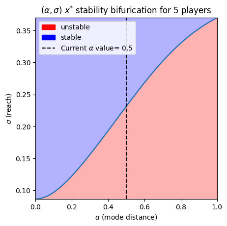
- first_order_bifurcation_plot(processed_data, infl_type='gaussian', alpha_st=0, alpha_end=1, alpha_values=None, cutoff_index=None, title_ads=[], save=False, name_ads=[], font={'cbar_size': 16, 'default_size': 24, 'font_family': 'sans-serif', 'label_size': 10, 'legend_size': 12, 'table_size': 15, 'title_size': 34}, save_types=['.png', '.svg'], paper_figure={'figure_id': 'bif_diag', 'paper': False, 'section': '3_2_6'})#
Generate and plot first-order bifurcation diagram with stability analysis.
This method creates a visualization of first-order (saddle-node) bifurcations by computing equilibrium positions and their stability across a parameter range. The plot shows how equilibrium agent positions change as a resource parameter (alpha) varies, with stability indicated through
InflGame.adaptive.jacobian.jacobian_stability_fast.The method supports both original format (e.g., Gaussian kernels) and processed data format with pre-computed stability flips, making it flexible for different analysis workflows.
First-order bifurcations are characterized by the creation or annihilation of equilibrium pairs, typically visualized as branches that meet and disappear at critical parameter values.
Example Gaussian Bifurcation Diagram
First-order bifurcation plot for 5 players using symmetric Gaussian influence kernels.#
- Parameters:
- infl_typestr
Type of influence kernel (‘gaussian’, ‘beta’, etc.).
- alpha_stfloat
Starting value of the resource parameter range.
- alpha_endfloat
Ending value of the resource parameter range.
- processed_dataOptional[dict]
Pre-processed bifurcation data with ‘unstable_flip’, ‘stable_flip’, and optionally ‘cycles_end’.
- alpha_valuesOptional[np.ndarray]
Array of alpha (parameter) values corresponding to equilibria.
- cutoff_indexOptional[int]
Index to truncate the data (useful for focusing on specific parameter ranges).
- title_adsList[str]
Additional text to append to plot title.
- savebool
Whether to save the plot to file.
- name_adsList[str]
Additional text for saved filename.
- fontDict
Font configuration dictionary with keys: ‘default_size’, ‘cbar_size’, ‘title_size’, ‘legend_size’, ‘table_size’, ‘label_size’, ‘font_family’.
- save_typesList[str]
List of file formats for saving (e.g., [‘.png’, ‘.svg’]).
- paper_figuredict
Configuration for paper figure saving with keys: ‘paper’ (bool), ‘section’ (str), ‘figure_id’ (str).
- Returns:
- matplotlib.figure.Figure
The generated matplotlib figure object.
Examples
fig = bif_env.first_order_bifurcation_plot(
    infl_type='gaussian',
    alpha_st=0.0,
    alpha_end=1.0,
    save=True,
    name_ads=['my_bifurcation'],
    title_ads=['3-Player System']
)
fig.show()
- learning_rate_large_end(resource_parameter, second_run=False, high_end=False)#
Determine appropriate learning rate upper bound for bifurcation analysis.
This method computes an appropriate maximum learning rate for gradient ascent based on the resource parameter value, with adjustments for refinement runs. The learning rate is scaled to ensure convergence while maintaining computational efficiency across different parameter regimes.
- Parameters:
- resource_parameterfloat
Current value of the resource/reach parameter.
- second_runbool
Whether this is a refinement run (uses larger learning rate if True).
- high_endbool
Whether this is for high parameter values (further increases learning rate).
- Returns:
- float
Computed maximum learning rate value.
- setup_adaptive_env()#
Set up the adaptive environment for bifurcation analysis.
This method initializes the gradient function environment with the provided parameters, creating an
InflGame.adaptive.grad_func_env.AdaptiveEnvinstance that will be used for equilibrium computations and bifurcation analysis.- Returns:
- None